Relational Data Modeling
Learn how to use relations to model data.
Introduction
Models
Physical Models
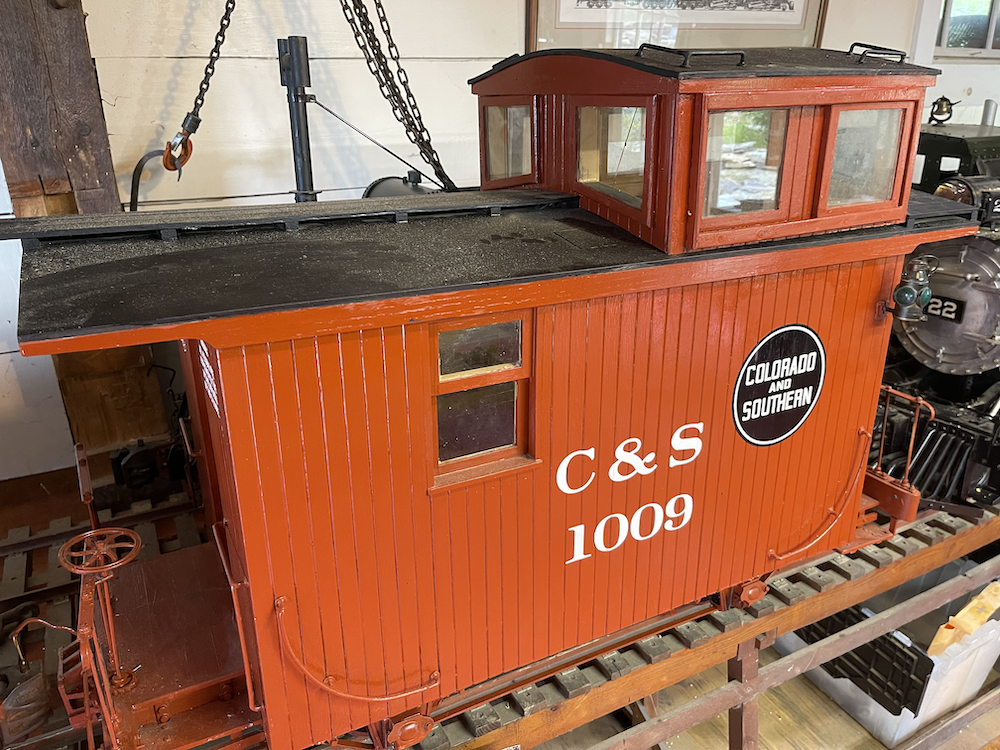
A model train is a physical object designed to be similar in some respects to a real train. The similarities between the model and the train are useful for drawing conclusions about the train based on features of the model. For example, an observer may conclude that the train car being represented by this model has several windows:
In general, a physical model consists of three parts:
- The original object.
- The model object.
- A correspondence between some aspects of the original and aspects of the model.
For example, the color of the model, the shapes of its windows, and the letters on the side match corresponding features of the original. Other features of the original, like its size, material composition, and internal engineering details, do not have corresponding elements in the model.
A model train’s value comes from both similarities and differences to the original train. Its simplified internal structure makes it more affordable than a real train, and its small size makes it suitable for display in a home or museum. In general, people who build models aim to achieve an appropriate balance between fidelity and practicality.
Data Models
Real trains and model trains are both made of physical material, but not all models are physical. Many models used in day-to-day life are conceptual models of objects, phenomena, or situations.
For example, suppose you have been invited to a wedding out of town and are looking to book accommodation for the evening. A typical first step would be to collect information about hotels in the area and organize it in a table:
| name | stars | rate | gym |
|---|---|---|---|
| Courtyard | 3 | $159 | true |
| Grand Bohemian | 4 | $346 | true |
| Residence Inn | 3 | $154 | false |
| DoubleTree | 3 | $122 | false |
| Holiday Inn | 3 | $128 | true |
| Clarion Inn | 2 | $77 | false |
While you could say that your table is a model made of ink or pixels, it is more helpful to think of it as a presentation of a model made of concepts. Each hotel is represented in your model as a collection that includes a string (opens in a new tab), a number, a monetary amount, and a true/false value.
Collections, strings, numbers, monetary amounts, true, and false are all concepts rather than physical objects, so this model is indeed conceptual rather than physical. Furthermore, strings, numbers, monetary amounts, and true/false values are all data, so this model may be described more specifically as a data model1.
The elements of your data model are similar to actual hotels in only certain respects. Not only is plenty of information missing from the model, such as parking, laundry, mattress sizes, etc., but a real hotel is a place where you can actually spend the night. The same would not be true of a data model no matter how much information it represented. Nevertheless, the correspondence between the hotel model and the hotel is rich enough to help you with your search.
In general, a data model comprises three parts:
- A real-world object or phenomenon to be modeled.
- The conceptual structure of the data being used as a model.
- The set of rules defining the correspondence between the values in the model and features of the object or phenomenon being modeled.
Each hotel in the table is represented as a collection of four values. The table itself represents a set of such four-value collections. These aspects of the model constitute its conceptual — or mathematical — structure.
Furthermore, detailed information about the meaning of each column is needed to interpret the values in this table or to add a new row to the table. For example, perhaps the first value is the name of the hotel as it appears on Google Maps, the second value is the star rating reported by AAA, and so on. These rules describe how the data elements correspond to things in the real world.
Relation Terminology
Tables and Relations
The table provides a convenient way to visualize the data model you are using for your hotel search, but it has some features that are not essential to the model. For example, the data model would remain the same if you changed cosmetic features like the colors of the cells or the alignment of the text within each cell. Likewise, rearranging the rows would not change the data model, because no meaning has been assigned to the order of the rows. You could even dispense with the table altogether and write out the rows in plain text, perhaps like this:
- name: Courtyard
  stars: 3
  rate: $159
  gym: true
- name: Grand Bohemian
  stars: 4
  rate: $346
  gym: true
- name: Residence Inn
  stars: 3
  rate: $154
  gym: false
- name: DoubleTree
  stars: 3
  rate: $122
  gym: false
- name: Holiday Inn
  stars: 3
  rate: $128
  gym: true
- name: Clarion Inn
  stars: 2
  rate: $77
  gym: false
To help distinguish the essential features of the table from inessential ones, it’s customary to use mathematical vocabulary rather than table-specific vocabulary to describe the conceptual objects that make up the model. The four-element collections representing each hotel are called tuples. A set of tuples is called a relation. In other words, every row in the table represents a tuple, and the entire table represents a relation.
Reordering a table’s rows, for example, constitutes a change to the table, but it does not change the underlying relation. Removing a column from a table would change both the table and the relation it represents.
Templates and Fields
One helpful way to communicate how a relation should be interpreted is to supply a sentence template with blanks to be filled in with the elements of each tuple. For example, the following would be an appropriate template for the relation above:
[hotel] is a [stars]-star hotel with a nightly rate of [rate] dollars, and it [has | does not have] a gym.
The blanks in the template are called fields. Each field may be identified using a name, and the field names may be used as column headers in a tabular representation of the relation. For example, the third blank is the rate field in this relation.
Databases
A typical application involves several different kinds of facts. For example, if you want to investigate each hotel’s reviews in more detail, you may want a relation whose template is:
[hotel] received a [rating]-star review from [user].
The table for this template looks like this:
| hotel | rating | user |
|---|---|---|
| Courtyard | 5 | Jennifer Lanza |
| Courtyard | 5 | Taylor Glass |
| Grand Bohemian | 5 | Hannah Price |
| Residence Inn | 4 | Chris Colotti |
| Residence Inn | 2 | Nicholas Brown |
| Residence Inn | 3 | Kristine Fitts |
| Clarion Inn | 3 | Travis Kisner |
| ⋮ | ⋮ | ⋮ |
A collection of one or more relations is called a relational database. The relations’ tuples are called the database’s data. Everything else, including relation names, field names, and any other information that may be used to interpret or manage the data, is called the database’s schema.
Only a few rows are shown in the review table above because the actual relation would have thousands of tuples.
While you could use a pencil-and-paper approach for the original six-row relation, you would need to use software to analyze the much larger review relation.
An application designed to robustly store and query relational databases is called a Relational Database Management System (RDBMS).
Popular RDBMSs include PostgreSQL, Oracle, Snowflake, and BigQuery.
Normal Forms
Relational database design involves more than just arranging data into tables. For example, spreadsheet applications are built around the idea of creating tables, but their high degree of flexibility means that users must exercise care to ensure that their sheets are well organized and amenable to computation.
This section introduces some of the most important principles for designing schemas that are conceptually clear and that make it easy for RDBMSs to perform computations effectively.
First Normal Form
Suppose you want to put the ratings into the hotel table.
One way to do that is to create a new column called review whose cells store a list of rating values:
| name | stars | rate | gym | ratings |
|---|---|---|---|---|
| Courtyard | 3 | $159 | true | [5, 5] |
| Grand Bohemian | 4 | $346 | true | [5] |
| Residence Inn | 3 | $154 | false | [4, 2, 3] |
| DoubleTree | 3 | $122 | false | [] |
| Holiday Inn | 3 | $128 | true | [] |
| Clarion Inn | 2 | $77 | false | [3] |
For simplicity, this table only reflects the rows shown in the review table above. If the actual review table were used instead, each list would contain hundreds of values.
This design is generally regarded as undesirable or impermissible because the possibility of having a list as an entry makes it more difficult to specify queries and reason about the contents of the table.
For example, with the original two-relation schema, the query “Which hotels have at least one two-star review?” is a relation-level operation that can be expressed and computed efficiently with any RDBMS.
With the one-relation schema containing ratings in a list, the query mixes cell-level calculations — searching for a value in a list — with relation-level calculations — identifying tuples that meet a condition. While some RDBMSs, including PostgreSQL, do allow this behavior, it comes at the cost of considerable complexity because database users have to learn different techniques for cell-level and relation-level calculations.
In summary, a database schema should require every element of every tuple to contain a single value, like a date, string, or number. A database whose schema satisfies this property is in First Normal Form (1NF).
Putting a table into 1NF usually requires splitting it into multiple tables. In this example, the ratings column must be separated into its own table. Here’s an example of how that may be done:
| name | stars | rate | gym |
|---|---|---|---|
| Courtyard | 3 | $159 | true |
| Grand Bohemian | 4 | $346 | true |
| Residence Inn | 3 | $154 | false |
| DoubleTree | 3 | $122 | false |
| Holiday Inn | 3 | $128 | true |
| Clarion Inn | 2 | $77 | false |
| position | hotel | rating |
|---|---|---|
| 1 | Courtyard | 5 |
| 2 | Courtyard | 5 |
| 1 | Grand Bohemian | 5 |
| 1 | Residence Inn | 4 |
| 2 | Residence Inn | 2 |
| 3 | Residence Inn | 3 |
| 1 | Clarion Inn | 3 |
| ⋮ | ⋮ | ⋮ |
Note: The second table includes the index of each rating within its array because that approach preserves all of the information in the non-1NF table. Other approaches, like identifying each rating by the user who submitted it, are also fine.
Keys and Values
The definitions for all of the normal forms beyond 1NF make reference to relations’ keys and value fields, so this section introduces those terms.
Keys
Each row in the hotels table is uniquely determined by the hotel identifier in the first column because each hotel has a specific star rating, nightly rate, and gym status:
| name | stars | rate | gym |
|---|---|---|---|
| Courtyard | 3 | $159 | true |
| Grand Bohemian | 4 | $346 | true |
| Residence Inn | 3 | $154 | false |
| DoubleTree | 3 | $122 | false |
| Holiday Inn | 3 | $128 | true |
| Clarion Inn | 2 | $77 | false |
A field that can be uniquely determined by another field or set of fields is said to be functionally dependent on that field or set of fields.
For example, stars, rate, and gym are functionally dependent on name.
In the review table, a row is uniquely identified by its hotel and user fields, since a user is not allowed to provide two different star ratings for the same hotel:
| hotel | rating | user |
|---|---|---|
| Courtyard | 5 | Jennifer Lanza |
| Courtyard | 5 | Taylor Glass |
| Grand Bohemian | 5 | Hannah Price |
| Residence Inn | 4 | Chris Colotti |
| Residence Inn | 2 | Nicholas Brown |
| Residence Inn | 3 | Kristine Fitts |
| Clarion Inn | 3 | Travis Kisner |
| ⋮ | ⋮ | ⋮ |
The hotel field does not uniquely identify a row, since each hotel may have multiple reviews.
The hotel and rating fields together also do not uniquely identify a row, since multiple users may give the same star rating to the same hotel.
A field or set of fields that can be used to uniquely identify tuples in a relation is called a key.
For example, the name field is the key of the hotels table, while the key of the reviews table consists of the hotel and user fields.2
It is possible for a relation to have more than one key. For example, consider a table of students with a Student ID column as well as a Social Security Number column. Since either of these two numbers uniquely identifies a student, either column can serve as a key. In such cases, a primary key may be chosen and declared.
Values
The fields that are not part of the key are called value fields.
The hotels table has three value fields, and the review table has one value field.
It is possible for a relation to have no value fields. For example, consider a relation that records the hotel stays that you have paid for:
| date | hotel |
|---|---|
| 2019-11-10 | Hotel Hive |
| 2019-12-22 | Treehouse Hotel London |
| 2019-12-23 | Treehouse Hotel London |
| 2022-04-18 | Hilton Garden Inn Denver |
| ⋮ | ⋮ |
This table’s key includes both fields because it’s possible to pay for two hotel bookings for the same date, and it’s possible to pay for multiple evenings at the same hotel.
Third Normal Form
Suppose that you want to consider the loyalty program points that you can get for your wedding hotel stay. Some of the hotels are part of a hotel chain, and each chain has its own loyalty program:
| name | chain | program |
|---|---|---|
| Courtyard | Marriott | Bonvoy |
| Residence Inn | Marriott | Bonvoy |
| DoubleTree | Hilton | Honors |
| Holiday Inn | IHG | IHG |
The third column in this table is functionally dependent on the second column.
In other words, each row’s program value may be determined by looking at its chain value.
This introduces the possibility of data inconsistency.
For example, suppose that Marriott changes its rewards program and that only one of the first two rows in this table is correctly updated. Then the database would be unclear on which rewards program Marriott participates in.
If, instead, the chain-program relationship is split into its own table, there is no such potential for inconsistency:
| name | chain |
|---|---|
| Courtyard | Marriott |
| Residence Inn | Marriott |
| DoubleTree | Hilton |
| Holiday Inn | IHG |
| chain | program |
|---|---|
| Marriott | Bonvoy |
| Hilton | Honors |
| IHG | IHG |
If an errant change were made under this schema, the data might be incorrect, but they could not be inconsistent. In other words, each fact encoded by this collection of relations is recorded in only one place.
Not all functional dependencies are a problem.
The rating field is functionally dependent on hotel and user in the table below, and this does not introduce any potential for inconsistency:
| hotel | rating | user |
|---|---|---|
| Courtyard | 5 | Jennifer Lanza |
| Courtyard | 5 | Taylor Glass |
| Grand Bohemian | 5 | Hannah Price |
| Residence Inn | 4 | Chris Colotti |
| Residence Inn | 2 | Nicholas Brown |
| Residence Inn | 3 | Kristine Fitts |
| Clarion Inn | 3 | Travis Kisner |
| ⋮ | ⋮ | ⋮ |
The difference between this example and the undesirable loyalty program example is that in this case the dependency is on the relation’s key. The dependency of a value field on the key is necessary.
A collection of tables is said to be in Third Normal Form (3NF) if the only functional dependencies are the ones for which a value field in a relation is functionally dependent on that relation’s key. Any other functional dependency should be avoided:
-
A functional dependency of a value field on another value field or fields.
Consider a
hoteltable with azip_codefield and astatefield. Thestatefield is functionally dependent on thezip_codefield, and both of them are value fields. Therefore, this table is not in 3NF. To put it in 3NF, remove thestatefield and create a separate relation to record each ZIP code’s state. -
A functional dependency of a value field on some of the key fields but not all of them.
Consider a
reviewtable with the fieldshotel,rating,user, anduser_review_count, with theuser_review_countfield recording the total number of reviews thatuserhas made on the site. Sinceuser_review_countcan be determined by theuserfield alone, this table is not in 3NF. To put it in 3NF, remove theuser_review_countfield and create a separate relation to record each user’s review count.
RDBMSs of all kinds encourage users to model data in 3NF.
Graph Normal Form
RelationalAI goes a step beyond most RDBMSs by encouraging schemas in which each relation has at most one value column. In RelationalAI terminology, such a database is said to be in Graph Normal Form3. A database in Third Normal Form may be put into Graph Normal Form by splitting every table with value columns into tables whenever is greater than :
def stars = {
  ("Courtyard", 3);
  ("Grand Bohemian", 4);
  ("Residence Inn", 3);
  ("DoubleTree", 3);
  ("Holiday Inn", 3);
  ("Clarion Inn", 2);
}

def rate = {
  ("Courtyard", 159);
  ("Grand Bohemian", 346);
  ("Residence Inn", 154);
  ("DoubleTree", 122);
  ("Holiday Inn", 128);
  ("Clarion Inn", 77);
}

def gym = {
  ("Courtyard", true);
  ("Grand Bohemian", true);
  ("Residence Inn", false);
  ("DoubleTree", false);
  ("Holiday Inn", true);
  ("Clarion Inn", false);
}
You can wrap a collection of commonly keyed relations in a module and display it as a table with more than one value column:
// read query

module hotel
  def stars = {
    ("Courtyard", 3);
    ("Grand Bohemian", 4);
    ("Residence Inn", 3);
    ("DoubleTree", 3);
    ("Holiday Inn", 3);
    ("Clarion Inn", 2);
  }

  def rate = {
    ("Courtyard", 159);
    ("Grand Bohemian", 346);
    ("Residence Inn", 154);
    ("DoubleTree", 122);
    ("Holiday Inn", 128);
    ("Clarion Inn", 77);
  }

  def gym = {
    ("Courtyard", true);
    ("Grand Bohemian", true);
    ("Residence Inn", false);
    ("DoubleTree", false);
    ("Holiday Inn", true);
    ("Clarion Inn", false);
  }
end

def output = table[hotel]
Wide Versus Tall Tables
This section addresses one final principle of relational database design.
Suppose that a company wants to record how many nights of hotel accommodation it books for each of its salespersons in each month. One approach is to put the data into a table whose columns correspond to months:
| name | Jan | Feb | Mar | Apr |
|---|---|---|---|---|
| Alice | 3 | 6 | 4 | 9 |
| Beatrice | 5 | 2 | 10 | 1 |
| Carlos | 4 | 4 | 5 | 3 |
On one hand, this method of organization makes a lot of sense: There are two axes — vertical and horizontal — and effectively two keys — person and month. The table makes full use of the available dimensions by using one key per axis.
However, standard relational database design principles disallow this setup because it causes the number of columns to grow in an open-ended way. Monthly changes to this table’s schema would need to be scheduled, and appropriate changes would need to be made for queries that involve this table.
In other words, it should be possible to make routine changes to data without changing the database’s schema, and this approach violates that principle.
Another approach is to use a tall, or long, table that records the same data with just three columns: name, month, and value.
In other words, the tall table’s row axis is used for both names and months.
This wide-to-tall transformation is sometimes called stacking (opens in a new tab).
| name | month | days |
|---|---|---|
| Alice | Jan | 3 |
| Alice | Feb | 6 |
| Alice | Mar | 4 |
| Alice | Apr | 9 |
| Beatrice | Jan | 5 |
| Beatrice | Feb | 2 |
| Beatrice | Mar | 10 |
| Beatrice | Apr | 1 |
| Carlos | Jan | 4 |
| Carlos | Feb | 4 |
| Carlos | Mar | 5 |
| Carlos | Apr | 3 |
The new data that come in each month can now be added by creating new rows rather than new columns. Furthermore, moving the month names from the schema level to the data level makes it easier to formulate questions like “For which months does the table have data?” or “How many times was a person on the road for more than 10 nights in a month?”
For these reasons, tall tables are considered better relational database design.
Querying Relational Data
Organizing and storing data in relations is only part of what an RDBMS is expected to do. The system must also be able to retrieve data when it’s needed. Since it would be very inefficient in most cases for the system to retrieve entire tables, the system must also provide a query language that users may use to specify which results they want.
There are a variety of relational query languages, and doing justice to any of them would be beyond the scope of this article. So, this section discusses the core operations supported by all RDBMSs.4
Filters
One of the reasons it makes sense to store relations in tall rather than wide form is that you can query a relation to obtain all of the rows that meet a given logical condition. For example, suppose you want to see Beatrice’s hotel night counts for months other than January. In Rel, you can do that like this:
// read query

def hotel_nights = {
  ("Alice", "Jan", 3);
  ("Alice", "Feb", 6);
  ("Alice", "Mar", 4);
  ("Alice", "Apr", 9);
  ("Beatrice", "Jan", 5);
  ("Beatrice", "Feb", 2);
  ("Beatrice", "Mar", 10);
  ("Beatrice", "Apr", 1);
  ("Carlos", "Jan", 4);
  ("Carlos", "Feb", 4);
  ("Carlos", "Mar", 5);
  ("Carlos", "Apr", 3);
}

def output = {
    name, month, nights :
        hotel_nights(name, month, nights) and
        month != "Jan" and
        name = "Beatrice"
}
Getting a subset of the rows of a relation based on a logical condition applied to each tuple is called filtering. The ability to perform this operation in a general and efficient way is a powerful feature of RDBMSs because achieving similar functionality in nonrelational systems often requires quite a bit of planning and work.
Joins
As illustrated in the examples in the Normal Forms section, splitting a table into two tables with fewer columns can be useful for data modeling. However, if you store related data in separate tables, you have to be able to recombine the data when necessary. This operation is called a join.
As discussed in the previous section, this table is not in Third Normal Form:
| name | chain | program |
|---|---|---|
| Courtyard | Marriott | Bonvoy |
| Residence Inn | Marriott | Bonvoy |
| DoubleTree | Hilton | Honors |
| Holiday Inn | IHG | IHG |
However, its contents may be put into 3NF by splitting them into these two tables:
| name | chain |
|---|---|
| Courtyard | Marriott |
| Residence Inn | Marriott |
| DoubleTree | Hilton |
| Holiday Inn | IHG |
| chain | program |
|---|---|
| Marriott | Bonvoy |
| Hilton | Honors |
| IHG | IHG |
To join these two tables and recover the original table, you can use the second table to look up the loyalty program for each chain. One helpful way to visualize this process is to position the rows of the two tables along the sides of a rectangle5:
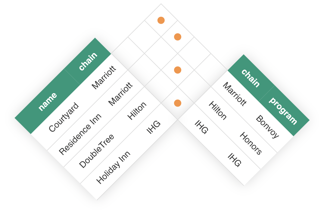
Each square in this figure represents a combination of a row from the first table and a row from the second table, and orange dots have been placed in the squares for which the chain values match for the two rows.
Each of these dots gives rise to one row in the joined table.
The resulting table is called a join of the two tables:
| name | chain | program |
|---|---|---|
| Courtyard | Marriott | Bonvoy |
| Residence Inn | Marriott | Bonvoy |
| DoubleTree | Hilton | Honors |
| Holiday Inn | IHG | IHG |
In general, joining two tables entails forming the product of the two tables, then potentially removing some of the resulting rows based on a condition applied to each row.6
One reason it’s useful to use a rectangle to visualize the join process, as opposed to thinking of the join as a lookup operation involving the second table, is that a row in one table may match no rows or multiple rows in the other table. The following figure shows a join of two hotel-chain tables based on whether the hotels belong to the same chain:
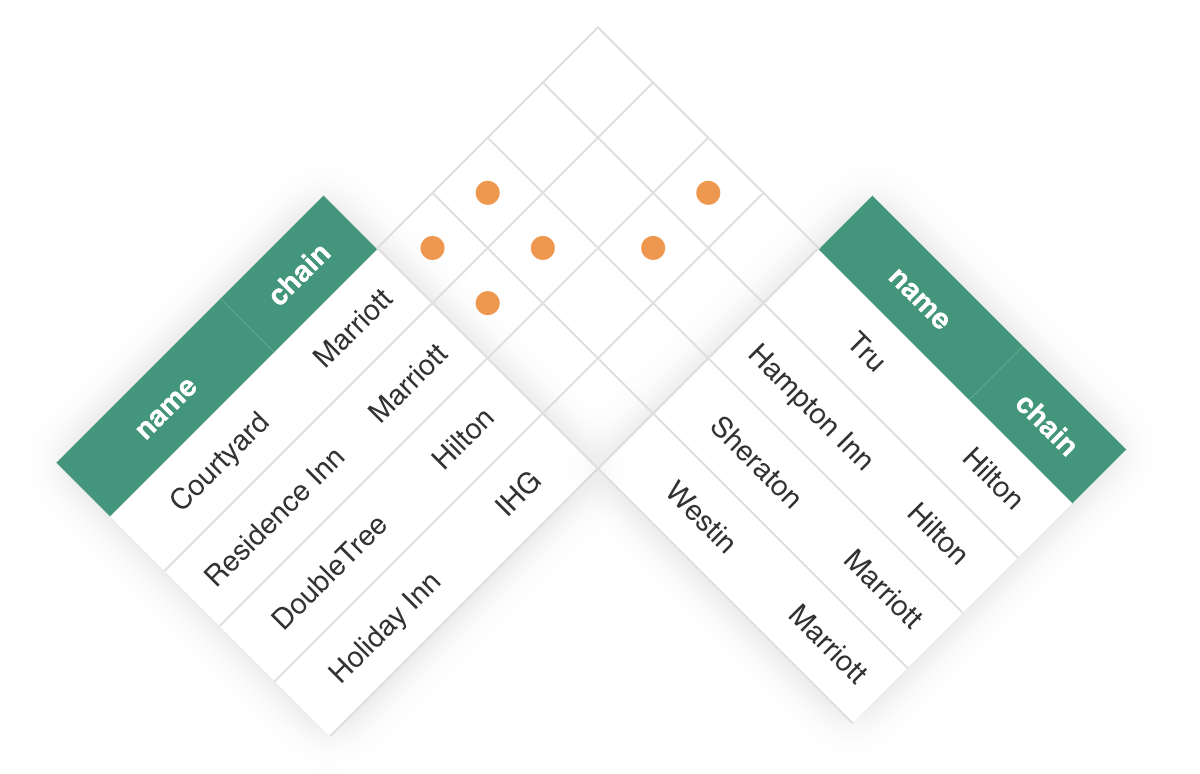
Each of the tables being joined has four rows, but the join has more than four rows because some rows match more than once. One row, namely the last row in the table on the left, doesn’t match any rows in the other table.7
Joins are often combined with a removal of some of the resulting columns.
You would want to remove one of the two chain columns in the animated figure above since the two columns are identical. Other columns may also be removed if they are not needed.
Other Operations
The other fundamental operations on relations are as follows:
- Union. Given two relations with the same fields, compute the relation consisting of all tuples that are in either of the two relations.
- Difference. Given two relations with the same fields, compute the relation consisting of all tuples that are in the first relation but not the second.
- Renaming. Change the names of relations and column header.
- Projection. Remove columns.
There are other operations often available in relational query systems that do not make the standard list of fundamental ones. For example, you can sort the tuples in a relation according to the values in a particular field. The result of such an operation is not really a relation since the order of its tuples must be considered meaningful. Nevertheless, sorting capabilities are typically provided by RDBMSs as a convenience.
Examples
This section illustrates how to use relations to model several common mathematical objects or real-world situations.
Irregular Tables
Many data sets encountered in the wild are organized into one large table, even when there are multiple kinds of facts to communicate. For example, here is the table published by the Massachusetts Bay Transit Authority for the outbound Providence Line train schedule:
| Station | Train 801 | Train 861 | Train 803 | Train 865 | Train 805 | Train 867 | Train 807 | Train 869 | Train 809 | Train 871 | Train 811 | Train 813 | Train 873 | Train 815 | Train 875 | Train 817 | Train 877 | Train 819 | Train 879 | Train 821 | Train 823 | Train 881 | Train 825 | Train 827 | Train 883 | Train 829 | Train 885 | Train 831 | Train 887 | Train 833 | Train 889 | Train 835 | Train 891 | Train 837 | Train 893 | Train 839 | ||
|---|---|---|---|---|---|---|---|---|---|---|---|---|---|---|---|---|---|---|---|---|---|---|---|---|---|---|---|---|---|---|---|---|---|---|---|---|---|---|
| bikes allowed | bikes allowed | bikes allowed | bikes allowed | bikes allowed | bikes allowed | bikes allowed | bikes allowed | bikes allowed | bikes allowed | bikes allowed | bikes allowed | bikes allowed | bikes allowed | bikes allowed | bikes allowed | bikes allowed | bikes allowed | bikes allowed | bikes allowed | bikes not allowed | bikes not allowed | bikes not allowed | bikes not allowed | bikes not allowed | bikes not allowed | bikes not allowed | bikes not allowed | bikes allowed | bikes allowed | bikes allowed | bikes allowed | bikes allowed | bikes allowed | bikes allowed | bikes allowed | |||
| South Station | parking | accessible | 4:25 AM | 5:25 AM | 6:25 AM | 7:00 AM | 7:25 AM | 8:00 AM | 8:25 AM | 8:57 AM | 9:25 AM | 10:00 AM | 10:25 AM | 11:25 AM | 12:05 PM | 12:25 PM | 1:05 PM | 1:20 PM | 2:05 PM | 2:25 PM | 2:55 PM | 3:25 PM | 3:52 PM | 4:00 PM | 4:25 PM | 4:52 PM | 5:00 PM | 5:40 PM | 6:00 PM | 6:22 PM | 7:00 PM | 7:25 PM | 8:00 PM | 8:25 PM | 9:00 PM | 9:40 PM | 10:20 PM | 11:00 PM |
| Back Bay | no parking | accessible | 4:30 AM | 5:30 AM | 6:30 AM | 7:05 AM | 7:30 AM | 8:05 AM | 8:30 AM | 9:02 AM | 9:30 AM | 10:05 AM | 10:30 AM | 11:30 AM | 12:10 PM | 12:30 PM | 1:10 PM | 1:25 PM | 2:10 PM | 2:30 PM | 3:00 PM | 3:30 PM | 3:57 PM | 4:05 PM | 4:30 PM | 4:57 PM | 5:05 PM | 5:45 PM | 6:05 PM | 6:27 PM | 7:05 PM | 7:30 PM | 8:05 PM | 8:30 PM | 9:05 PM | 9:45 PM | 10:25 PM | 11:05 PM |
| Ruggles | no parking | accessible | 4:33 AM | 5:33 AM | 6:33 AM | 7:08 AM | 7:33 AM | 8:08 AM | 8:33 AM | 9:05 AM | 9:33 AM | 10:08 AM | 10:33 AM | 11:33 AM | 12:13 PM | 12:33 PM | 1:13 PM | 1:28 PM | 2:13 PM | 2:33 PM | 3:03 PM | 3:33 PM | 4:01 PM | 4:08 PM | 4:33 PM | 5:01 PM | 5:08 PM | 5:49 PM | 6:08 PM | 6:30 PM | 7:08 PM | 7:33 PM | 8:08 PM | 8:33 PM | 9:08 PM | 9:48 PM | 10:28 PM | 11:08 PM |
| Forest Hills | parking | accessible | 11:13 PM | |||||||||||||||||||||||||||||||||||
| Hyde Park | parking | accessible | 9:41 AM | 10:16 AM | 11:41 AM | 12:21 PM | 1:21 PM | 2:21 PM | 8:16 PM | 9:16 PM | 10:36 PM | 11:18 PM | ||||||||||||||||||||||||||
| Route 128 | parking | accessible | 4:44 AM | 5:44 AM | 6:44 AM | 7:18 AM | 7:44 AM | 8:18 AM | 8:44 AM | 9:15 AM | 9:51 AM | 10:21 AM | 10:44 AM | 11:47 AM | 12:29 PM | 12:44 PM | 1:26 PM | 1:39 PM | 2:26 PM | 2:44 PM | 3:14 PM | 3:44 PM | 4:19 PM | 4:44 PM | 5:19 PM | 6:00 PM | 6:19 PM | 6:41 PM | 7:19 PM | 7:44 PM | 8:21 PM | 8:44 PM | 9:21 PM | 9:59 PM | 10:41 PM | 11:25 PM | ||
| Canton Junction | parking | accessible | 4:50 AM | 5:50 AM | 6:50 AM | 7:24 AM | 7:50 AM | 8:24 AM | 8:50 AM | 9:21 AM | 9:57 AM | 10:27 AM | 10:50 AM | 11:53 AM | 12:35 PM | 12:50 PM | 1:32 PM | 1:45 PM | 2:32 PM | 2:50 PM | 3:20 PM | 3:50 PM | 4:25 PM | 4:50 PM | 5:25 PM | 6:06 PM | 6:25 PM | 6:47 PM | 7:25 PM | 7:50 PM | 8:27 PM | 8:50 PM | 9:27 PM | 10:05 PM | 10:47 PM | 11:31 PM | ||
| Canton Center | parking | accessible | 5:53 AM | 7:27 AM | 8:28 AM | 9:28 AM | 10:30 AM | 12:38 PM | 1:35 PM | 2:35 PM | 3:24 PM | 4:28 PM | 5:29 PM | 6:29 PM | 7:29 PM | 8:30 PM | 9:30 PM | 10:50 PM | ||||||||||||||||||||
| Stoughton | parking | accessible | 6:01 AM | 7:36 AM | 8:37 AM | 9:37 AM | 10:38 AM | 12:46 PM | 1:43 PM | 2:43 PM | 3:34 PM | 4:39 PM | 5:40 PM | 6:39 PM | 7:37 PM | 8:38 PM | 9:38 PM | 10:58 PM | ||||||||||||||||||||
| Sharon | parking | accessible | 4:56 AM | 6:56 AM | 7:56 AM | 8:56 AM | 10:03 AM | 10:56 AM | 11:59 AM | 12:56 PM | 1:51 PM | 2:56 PM | 3:56 PM | 4:17 PM | 4:56 PM | 5:17 PM | 6:12 PM | 6:53 PM | 7:56 PM | 8:56 PM | 10:11 PM | 11:37 PM | ||||||||||||||||
| Mansfield | parking | accessible | 5:04 AM | 7:04 AM | 8:04 AM | 9:04 AM | 10:11 AM | 11:04 AM | 12:07 PM | 1:04 PM | 1:59 PM | 3:04 PM | 4:04 PM | 4:25 PM | 5:04 PM | 5:25 PM | 6:20 PM | 7:01 PM | 8:04 PM | 9:04 PM | 10:19 PM | 11:45 PM | ||||||||||||||||
| Attleboro | parking | accessible | 5:12 AM | 7:12 AM | 8:12 AM | 9:12 AM | 10:19 AM | 11:12 AM | 12:15 PM | 1:12 PM | 2:07 PM | 3:12 PM | 4:12 PM | 4:34 PM | 5:12 PM | 5:34 PM | 6:29 PM | 7:09 PM | 8:12 PM | 9:12 PM | 10:27 PM | 11:53 PM | ||||||||||||||||
| Providence | parking | accessible | 5:45 AM | 7:45 AM | 8:33 AM | 9:33 AM | 10:45 AM | 11:33 AM | 12:36 PM | 1:40 PM | 2:26 PM | 3:38 PM | 4:33 PM | 4:59 PM | 5:34 PM | 5:55 PM | 6:57 PM | 7:34 PM | 8:40 PM | 9:33 PM | 10:48 PM | 12:14 AM | ||||||||||||||||
| TF Green Airport | parking | accessible | 6:00 AM | 8:00 AM | 11:00 AM | 1:55 PM | 3:53 PM | 5:13 PM | 6:09 PM | 7:12 PM | 8:55 PM | 11:03 PM | ||||||||||||||||||||||||||
| Wickford Junction | parking | accessible | 6:18 AM | 8:15 AM | 11:18 AM | 2:10 PM | 4:10 PM | 5:31 PM | 6:31 PM | 7:28 PM | 9:10 PM | 11:20 PM |
The first row specifies whether bikes are allowed on each train, while the subsequent rows indicate train departure times. Therefore, the rows do not all fit the same fact template. This implies that the table does not correspond to a relation.
Furthermore, even if the bikes row were removed, the fact template for the remaining rows would be very unwieldy:
[station] [ has | does not have] parking, [is | is not] accessible, has a Train 801 departure at [time], has a Train 861 departure at [time], …
All of those train numbers should really be data; they should not be part of the schema. In other words, the problem with this table is that it’s in wide form rather than tall form.
The best way to create a relational data model with the same information as this table is to disregard the original table shape altogether and instead think about the kinds of facts that are represented. There are four basic types:
Train [number] allows bikes. [station] has parking. [station] is accessible. Train [number] arrives at [station] at [time].
Therefore, the information in the table may be modeled using four relations:
allows_bikes:
| train |
|---|
| 861 |
| 803 |
| 865 |
| 805 |
| 867 |
| ⋮ |
| 839 |
parking:
| station |
|---|
| South Station |
| Forest Hills |
| Hyde Park |
| Route 128 |
| Canton Junction |
| Canton Center |
| Stoughton |
| Sharon |
| Mansfield |
| Attleboro |
| Providence |
| TF Green Airport |
| Wickford Junction |
accessible
| station |
|---|
| South Station |
| Back Bay |
| Ruggles |
| Forest Hills |
| Hyde Park |
| Route 128 |
| Canton Junction |
| Canton Center |
| Stoughton |
| Sharon |
| Mansfield |
| Attleboro |
| Providence |
| TF Green Airport |
| Wickford Junction |
departure_time
| station | train | time |
|---|---|---|
| South Station | 801 | 4:25 AM |
| South Station | 861 | 5:25 AM |
| South Station | 803 | 6:25 AM |
| South Station | 865 | 7:00 AM |
| South Station | 805 | 7:25 AM |
| ⋮ | ⋮ | ⋮ |
| Wickford Junction | 827 | 6:31 PM |
| Wickford Junction | 829 | 7:28 PM |
| Wickford Junction | 833 | 9:10 PM |
| Wickford Junction | 837 | 11:20 PM |
If you want to print out the train schedule and display it in your home, the original table is preferable to these four tables. However, the four-relation model is much better for purposes of storing and querying the data in a database management system.
Nested Data
Applications often store data in nested data structures. For example, when you play a video game, some of the information about the state of your game might be stored in a form that looks like this:
{
  name: "Aniko",
  color: "green",
  power_ids: [117, 844, 512],
  levels: {
    1: {
      points: 10,
      tries: [0.4, 0.5, 0.4, 0.65, 0.8, 1.0]
    },
    2: {
      points: 8,
      tries: [0.1, 0.1, 0.25, 0.85, 1.0]
    },
    3: {
      points: 10,
      tries: [0.3, 0.2, 0.45, 0.85, 0.9, 1.0]
    },
    4: {
      points: 9,
      tries: [0.2, 0.1, 0.15, 0.6, 0.1, 0.2, 0.8, 0.9, 0.95, 1.0]
    }
  }
}
This object is meant to be interpreted as follows:
- Your character’s name is Aniko.
- Your avatar is green.
- Your powers are the ones whose IDs are 117, 844, and 512.
- On Level 1, you got 10 points after trying six times to complete the level. The first time you completed 40% of the level before failing and having to start over, then 50%, then 40% again, and so on.
- …
The term nested refers to the fact that any of the values may store further compound values inside it.
For example, the list of tries values is inside the value for a particular level number, which in turn is inside the levels value.
Such nesting behavior is not allowed for a relation in First Normal Form.
One of the most commonly used formats for passing data around on the internet is a nested data format called JSON. Some database management systems, like MongoDB, are built to support nested data models rather than relational data models. For these reasons, it is very common to encounter nested data sources in practice.
Despite the structural differences between nested data and relations, you can build a relational model for these data by thinking about the types of facts that are represented. One way to organize the facts in the object above into a collection of sentence templates is as follows:
The character’s [attribute] is [value]. The character has power [power]. The character earned [score] points on level [level]. On level [level] and try number [try] on that level, you completed [proportion] of the level.
The tables for these templates look like this:
| attribute | value |
|---|---|
| name | Aniko |
| color | green |
| power |
|---|
| 117 |
| 844 |
| 512 |
| level | points |
|---|---|
| 1 | 10 |
| 2 | 8 |
| 3 | 10 |
| 4 | 9 |
| level | try | proportion |
|---|---|---|
| 1 | 1 | 0.4 |
| 1 | 2 | 0.5 |
| 1 | 3 | 0.4 |
| 1 | 4 | 0.65 |
| 1 | 5 | 0.8 |
| 1 | 6 | 1.0 |
| 2 | 1 | 0.1 |
| ⋮ | ⋮ | ⋮ |
| 4 | 9 | 0.95 |
| 4 | 10 | 1.0 |
Graphs
Relationships between real-world entities may be represented graphically, with points representing the entities and labeled lines representing the relationships:
This figure represents a situation in which Alice and Beatrice are friends, Beatrice and Carlos are friends, Alice and Carlos aren’t friends, Alice is French and was born on 1996-04-17, and so on.
The points are called nodes or vertices, and pairs of nodes — indicated by the lines connecting them — are called relationships or edges. A set of vertices connected in pairs by edges is called a graph.
The graph representation is well-suited to problems for which it is important to understand how things are related to each other. For example, it’s visually apparent from the graph that Carlos is a second-degree friend of Alice — that is, a friend of a friend. Some organizations use Graph Database Management Systems, like Neo4j, to build their entire database on a graph-based data model.
It is straightforward to represent a graph database as a relational database because a graph is a collection of relations. Specifically, each edge represents a pair of nodes, and a pair is a two-element tuple. Therefore, each edge type gives rise to a relation containing two-element tuples:
def friends = {
  ("Alice", "Beatrice");
  ("Beatrice", "Alice");
  ("Beatrice", "Carlos");
  ("Carlos", "Beatrice");
}

def birthday = {
  ("Alice", 1996-04-17);
  ("Beatrice", 1975-08-11);
  ("Carlos", 1981-11-06);
}

def nationality = {
  ("Alice", "France");
  ("Beatrice", "United States");
  ("Carlos", "Costa Rica");
}
Time Series
A time series is a sequence of values that are each associated with a date or time. For example, you might keep track of the performance of a stock over time by checking its price at 4 p.m. every trading day and recording a data point with that date and price.
Time series may be represented as relations with two-element tuples of the form (timestamp, value):
def stock_price = {
  (2022-01-03, 617.05);
  (2022-01-04, 619.37);
  (2022-01-05, 618.11);
  (2022-01-06, 618.88);
}
Arrays
One-Dimensional Arrays
A one-dimensional array is an ordered sequence of values:
Since the tuples in a relation have no particular order, it does not work to represent an array as a relation of one-element tuples:
// read query

def A = {4; 18; 3; 11; 7}

def output = A
Instead, you can create a relation of two-element tuples with both the index and element:
// read query

def A = {
  (1, 4);
  (2, 18);
  (3, 3);
  (4, 11);
  (5, 7);
}

def output = A
Note: While tuples and arrays are both ordered sequences of values, you should not use a tuple to model an array in Rel, because the language is not designed to support that approach. Instead, use a collection of (index, value) pairs as described above.
Multidimensional Arrays
A similar approach works for multidimensional arrays. For example, consider this two-dimensional array:
The idea is to use a relation of three-element tuples of the form (row index, column index, value):
// read query

def A = {
  (1, 1, 24);
  (1, 2, 14);
  (1, 3, 11);
  (2, 1, 7);
  (2, 2, 8);
  (2, 3, 12);
  (3, 1, 5);
  (3, 2, 4);
  (3, 3, 9);
}

def output = A
This is sometimes called the “ijv” or “triplet” format for representing a two-dimensional array. You can access specific values using partial relational application:
// read query

def A = {
  (1, 1, 24);
  (1, 2, 14);
  (1, 3, 11);
  (2, 1, 7);
  (2, 2, 8);
  (2, 3, 12);
  (3, 1, 5);
  (3, 2, 4);
  (3, 3, 9);
}

def output = A[1, 2]
Hierarchies
The National Basketball Association has 30 teams, which are subdivided into two conferences of 15 teams each. Each conference is further subdivided into three divisions of five teams each. This is an example of a hierarchy, and it may be visualized using an outline:
- Eastern Conference
- Atlantic Division
- Boston Celtics
- New Jersey Nets
- New York Knicks
- Philadelphia 76ers
- Toronto Raptors
- Central Division
- Chicago Bulls
- Cleveland Cavaliers
- Detroit Pistons
- Indiana Pacers
- Milwaukee Bucks
- Southeast Division
- Atlanta Hawks
- Charlotte Bobcats
- Miami Heat
- Orlando Magic
- Washington Wizards
- Atlantic Division
- Western Conference
- Northwest Division
- Denver Nuggets
- Minnesota Timberwolves
- Oklahoma City Thunder
- Portland Trail Blazers
- Utah Jazz
- Pacific Division
- Golden State Warriors
- Los Angeles Clippers
- Los Angeles Lakers
- Phoenix Suns
- Sacramento Kings
- Southwest Division
- Dallas Mavericks
- Houston Rockets
- Memphis Grizzlies
- New Orleans Pelicans
- San Antonio Spurs
- Northwest Division
Despite the structural differences between an outline and a table, hierarchical relationships may be modeled very reasonably as relations. To build a relational model, consider the kinds of facts that are implicit in the outline and create a relation for each fact template.
In this case, there are relationships between divisions and conferences:
The Atlantic Division is in the Eastern Conference
The Central Division is in the Eastern Conference
The Southeast Division is in the Eastern Conference
The Northwest Division is in the Western Conference
The Pacific Division is in the Western Conference
The Southwest Division is in the Western Conference
The other kind of relationship is the one between teams and divisions:
The Boston Celtics are in the Atlantic Division
The New Jersey Nets are in the Atlantic Division
…
Therefore, the NBA’s conference and division hierarchy may be modeled using two relations:
| division | conference |
|---|---|
| Atlantic | Eastern |
| Central | Eastern |
| Southeast | Eastern |
| Northwest | Western |
| Pacific | Western |
| Southwest | Western |
| team | division |
|---|---|
| Boston Celtics | Atlantic |
| Brooklyn Nets | Atlantic |
| New York Knicks | Atlantic |
| Philadelphia 76ers | Atlantic |
| Toronto Raptors | Atlantic |
| Chicago Bulls | Central |
| ⋮ | ⋮ |
| New Orleans Pelicans | Southwest |
| San Antonio Spurs | Southwest |
Summary
In summary, relational data modeling is a flexible paradigm for representing facts in an organized way. The main idea is to create a collection of sentence templates that generalize the facts being represented. Each template gives rise to a relation whose tuples represent the ways that the template’s fields may be filled in to obtain a fact. A relational database is a collection of such relations.
The Normal Forms convey principles about how to split relations in such a way that redundancies are eliminated. Query operations allow you to retrieve data from the database, including filtering to obtain a subset of a relation’s tuples based on a logical condition and joins for combining data from multiple relations.
Footnotes
-
Not every conceptual model is a data model. For example, friendship between individuals may be posited as a conceptual model for alliance between countries. The concept of friendship is a model in this example, but it is not data. ↩
-
It should be understood in this definition that a key should not include more fields than necessary. For example, a row in the
reviewtable is uniquely determined by all three fields, but theratingfield should not be included in the key since a row is also uniquely determined by just thehotelanduserfields. ↩ -
Graph Normal Form has a second requirement, which is that values in the database should be equal if and only if they are meant to correspond to the same thing in the real world. For more details, see the Graph Normal Form concept guide. ↩
-
The designation of these specific operations as the fundamental ones goes back to Ted Codd’s paper A Relational Model of Data for Large Shared Data Banks, which was published in Communications of the ACM in June of 1970. ↩
-
Visualization credit: R for Data Science (opens in a new tab). ↩
-
The steps actually performed by database systems are often quite different from these steps because it’s often possible to achieve mathematically identical results with less work. ↩
-
In some cases, it may be necessary to keep track of rows in one table that do not match any rows in the other table. This is customarily done by adding a single row to the joined table for the unmatched row, with missing values for all of the fields from the other table.
In a left join, any unmatched rows from the first table are retained in this way. In a right join, any unmatched rows from the second table are retained. In a full join, any unmatched rows from either table are retained.
These variations of the join operation are not necessary in Rel because unmatched rows may be handled using separate logic. ↩