Debugging

The RelationalAI (RAI) Debugger is a browser-based tool that ships with the relationalai Python package. You can use it to identify issues with your model, such as incorrect query results, slow query performance, or unexpected behavior.

Caution

Currently, the RAI Debugger is only available when using the relationalai package in a local Python environment. Snowflake notebooks and other cloud environments do not support the RAI Debugger.

Tutorial: Use the Debugger

This tutorial walks you through the steps to open the RAI debugger, connect a program to it, and interact with the debugger interface. You’ll create a model with some bugs and use the debugger to identify and fix them.

Note

See Understand the Debugger Interface for detailed information about the interface components introduced in the tutorial.

Set Up Your Environment

To use the RAI Debugger, you need to have a local Python environment with the relationalai package installed:

macOS/Linux

# Create a new project folder.
mkdir my_project
cd my_project

# Create a new virtual environment.
# NOTE: Use the python3.9 or python3.10 command if you're using a different version of Python.
python3.11 -m venv .venv

# Activate the virtual environment.
source .venv/bin/activate

# Update pip and install the relationalai package.
# NOTE: python -m ensures that the pip command is run for your virtual environment.
python -m pip install -U pip
python -m pip install relationalai

Windows

# Create a new project folder.
mkdir my_project
cd my_project

# Create a new virtual environment.
python -m venv .venv

# Activate the virtual environment.
.\.venv\Scripts\activate

# Upgrade pip and install the relationalai package.
# NOTE: python -m ensures that the pip command is run for your virtual environment.
python -m pip install -U pip
python -m pip install relationalai

Start The Debug Server

Run the following command in your terminal to start the RAI Debugger server:

rai debugger

Tip

If you encounter an error about the rai command not being found, you may need to activate your project’s virtual environment or install the relationalai package.

Tip

If you encounter an error that says address already in use, then something is already running on the default port used by the debug server. You can specify a different port using the --port option:

rai debugger --port 1234

A new tab opens in your default browser to display the debugger interface:

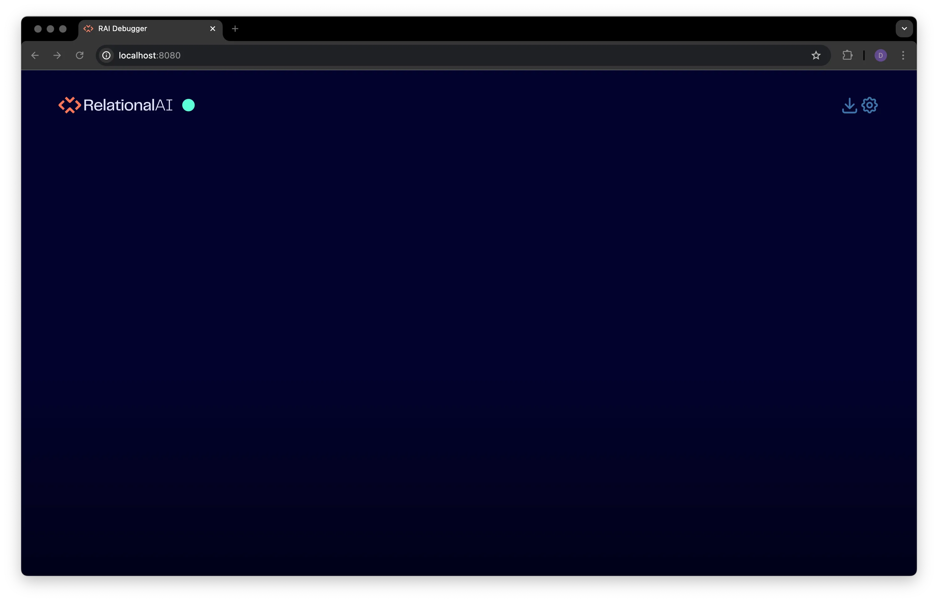
When it first opens, the debugger interface is empty. As you execute Python applications or Jupyter notebooks that use the relationalai package, the interface updates to show the execution timeline for the program.

Programs automatically connect to the debug server over the local network, unless their configuration sets the debug configuration key to False. Multiple programs can be viewed in the same debugger window simultaneously. See Multiple Connections for details.

Tip

If a raiconfig.toml file is detected in the current working directory, the debugger will check the connection configuration for the active profile.

The green dot next to the RelationalAI logo in the top left corner indicates that the debugger is able to connect to the configured RAI Native App. If the dot isn’t green, check that your configuration is correct and restart the debug server.

See the Configuration guide for details.

Customize The Debug Host and Port (Optional)

If necessary, you can change the host name and port used by the debug server by:

• Using the --host and --port options when running the rai debugger CLI command

• Setting the debug.host and debug.port configuration keys in your raiconfig.toml file.

CLI

rai debugger --host my_host --port 1234

raiconfig.toml

debug = true
debug.host = "my_host"  # default is "localhost"
debug.port = 1234  # default is 8080
active_profile = "default"

[profile.default]
user = <SNOWFLAKE_USER>
password = <SNOWFLAKE_PASSWORD>
account = <SNOWFLAKE_ACCOUNT_ID>
role = <SNOWFLAKE_ROLE>
warehouse = <SNOWFLAKE_WAREHOUSE>

Using the values from the custom configuration above, you’d point your browser to <my_host>:1234 to view the debugger interface.

View a Program’s Execution Timeline in the Debugger

Follow these steps to view a program in the debugger:

1. Create a model.

   In a file named my_project/model.py, create a file with the following code:

   my_project/model.py

   import relationalai as rai
   from relationalai.std import as_rows
   
   
   PERSON_DATA = [
         {"id": 1, "name": "Alice"},
         {"id": 2, "name": "Bob"},
         {"id": 3, "name": "Carol"},
   ]
   
   
   # Create a Model object.
   model = rai.Model("MyModel")
   Person = model.Type("Person")
   
   # Add data to the types from the hardcoded data.
   with model.rule():
         data = as_rows(PERSON_DATA)
         Person.add(id=data.id).set(name=data.name)
   
   # Query the data.
   with model.query() as select:
         person = Person()
         response = select(person.id, person.name)
   
   print(response.results)

2. Run the program.

   In a separate terminal window, activate your project’s virtual environment and then run the model.py file:

   # Activate the virtual environment. On macOS/Linux, use:
   source venv/bin/activate
   
   # On Windows, use:
   .\venv\Scripts\activate
   
   # Execute the model.py file with Python.
   python model.py

   Note

   You may notice that a debug.jsonl file is created in the directory from which you ran the program. This file contains raw debug logs generated by the program. See The debug.jsonl File for details.

3. View the execution timeline.

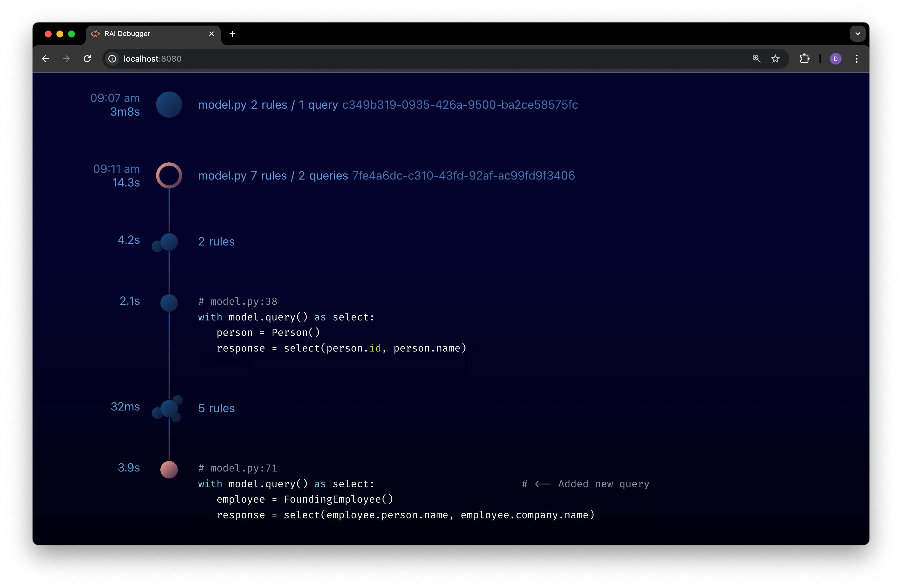
   In the debugger interface, you’ll see a timeline of the model’s execution:

   

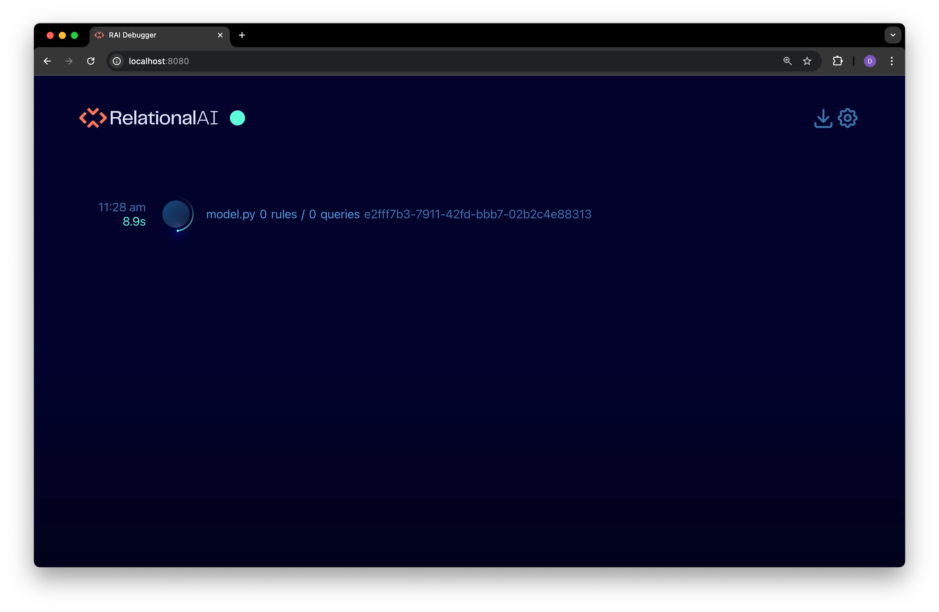
   As the model executes, the timeline updates to show the execution events in chronological order:

   

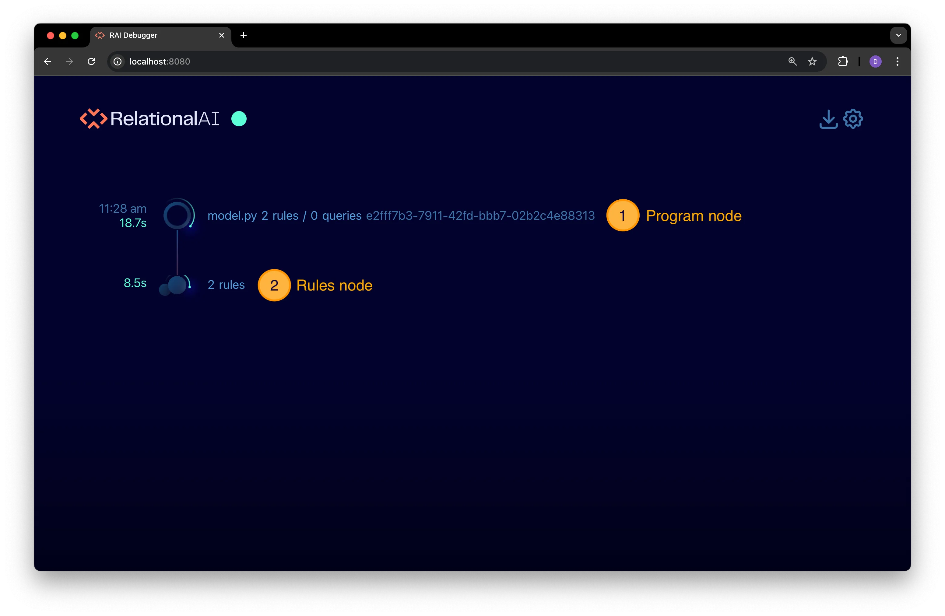
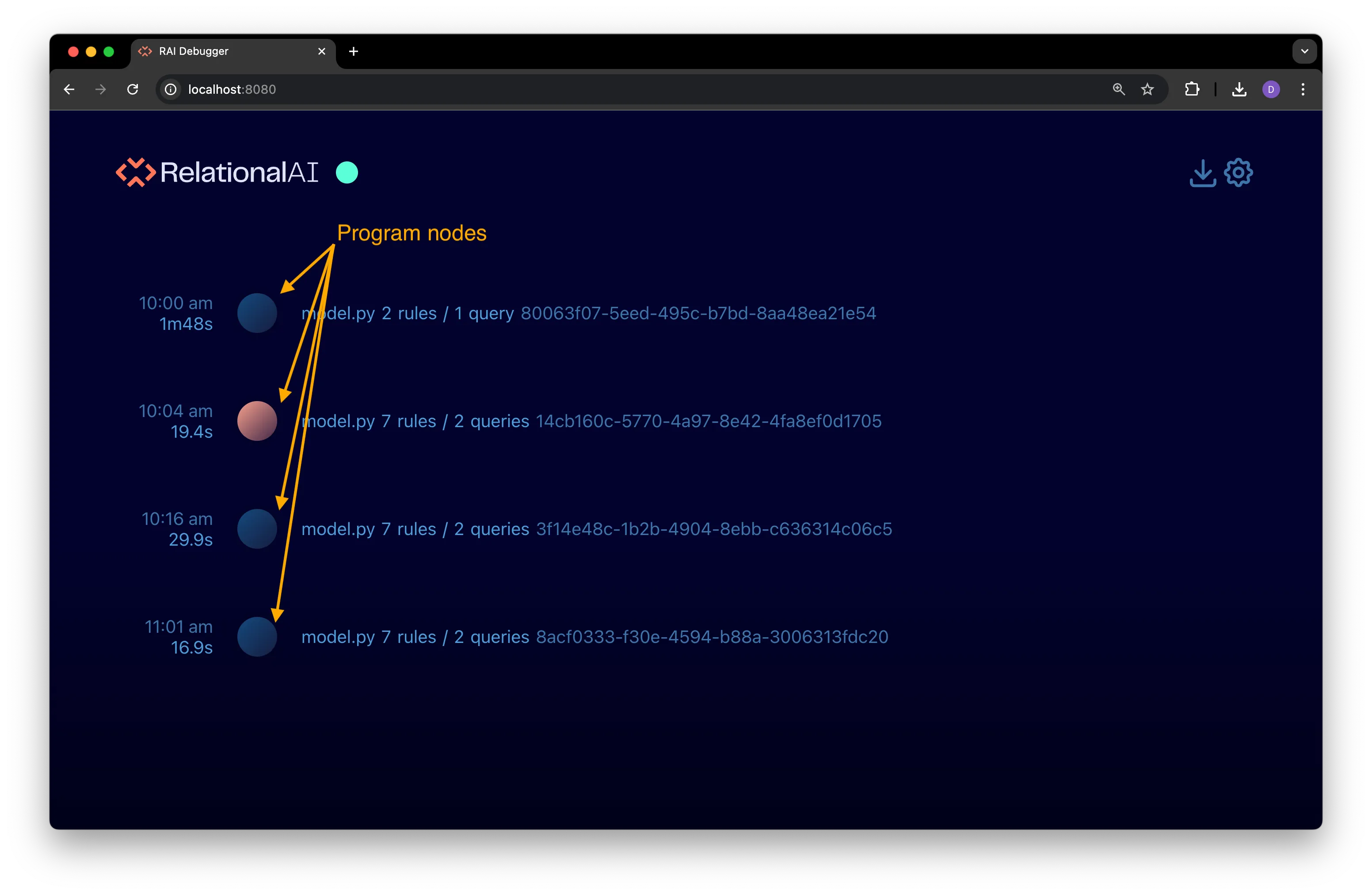
   In the timeline:

   • Each event is displayed as a node in the timeline.
   • An event’s elapsed execution time is shown to the left of it’s timeline icon.
   • Events currently being executed are indicated by an animated spinner around it’s timeline that disappears when execution is complete.

   The timeline in the preceding figure has two event nodes:

   1. A program node that represents the execution of a single program.

   2. A rules node that represents a set of compiled rules that are being installed in the model’s configured RAI engine as part of the RAI program lifecyle.

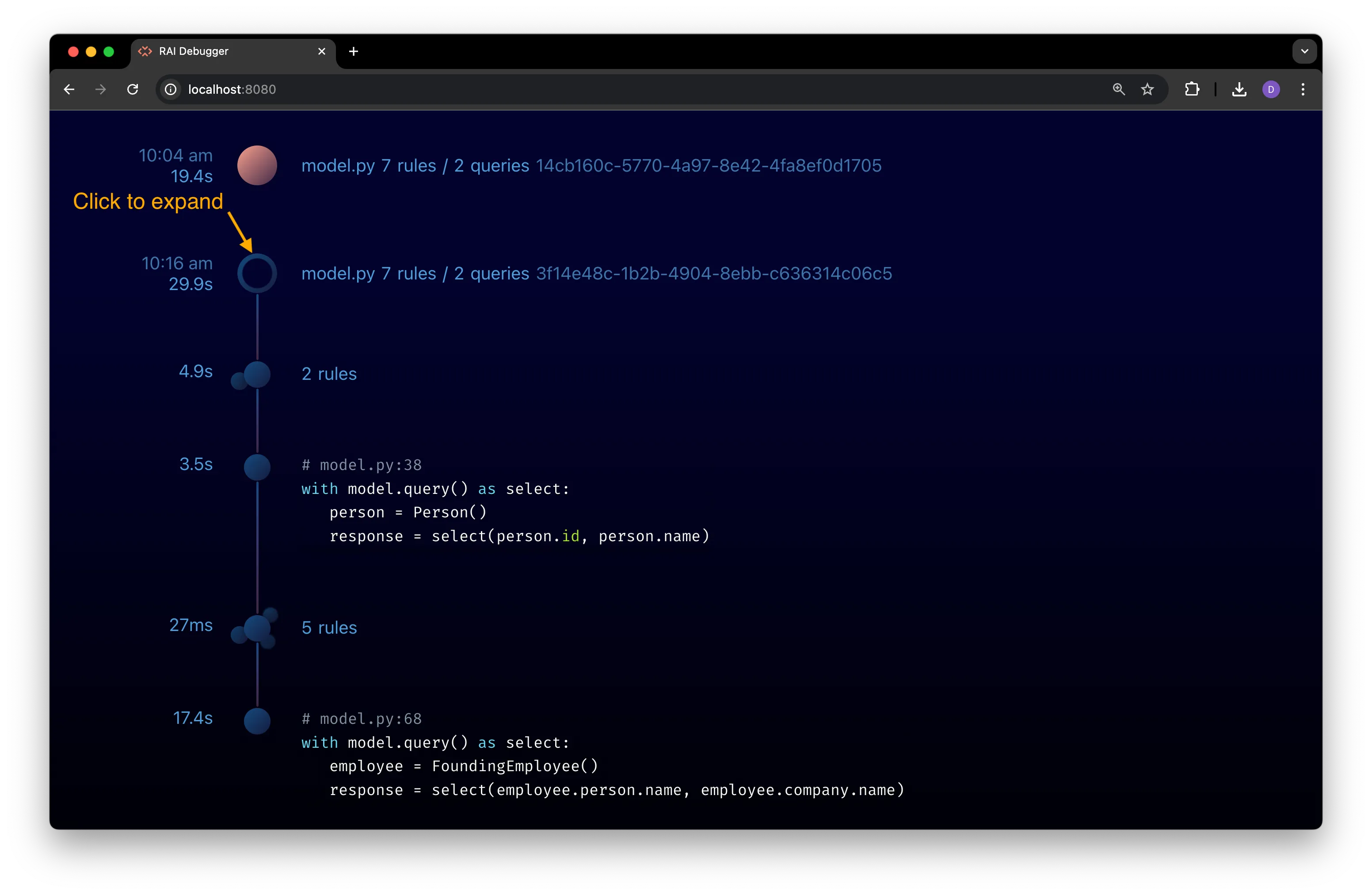
4. Collapse and expand the program node.

   Click on the program node’s timeline icon and it collapses to a compact view. The rules node disappears from the timeline because it gets folded up into its corresponding program node.

   Click the program node again to return to the expanded view.

5. Explore the rules node.

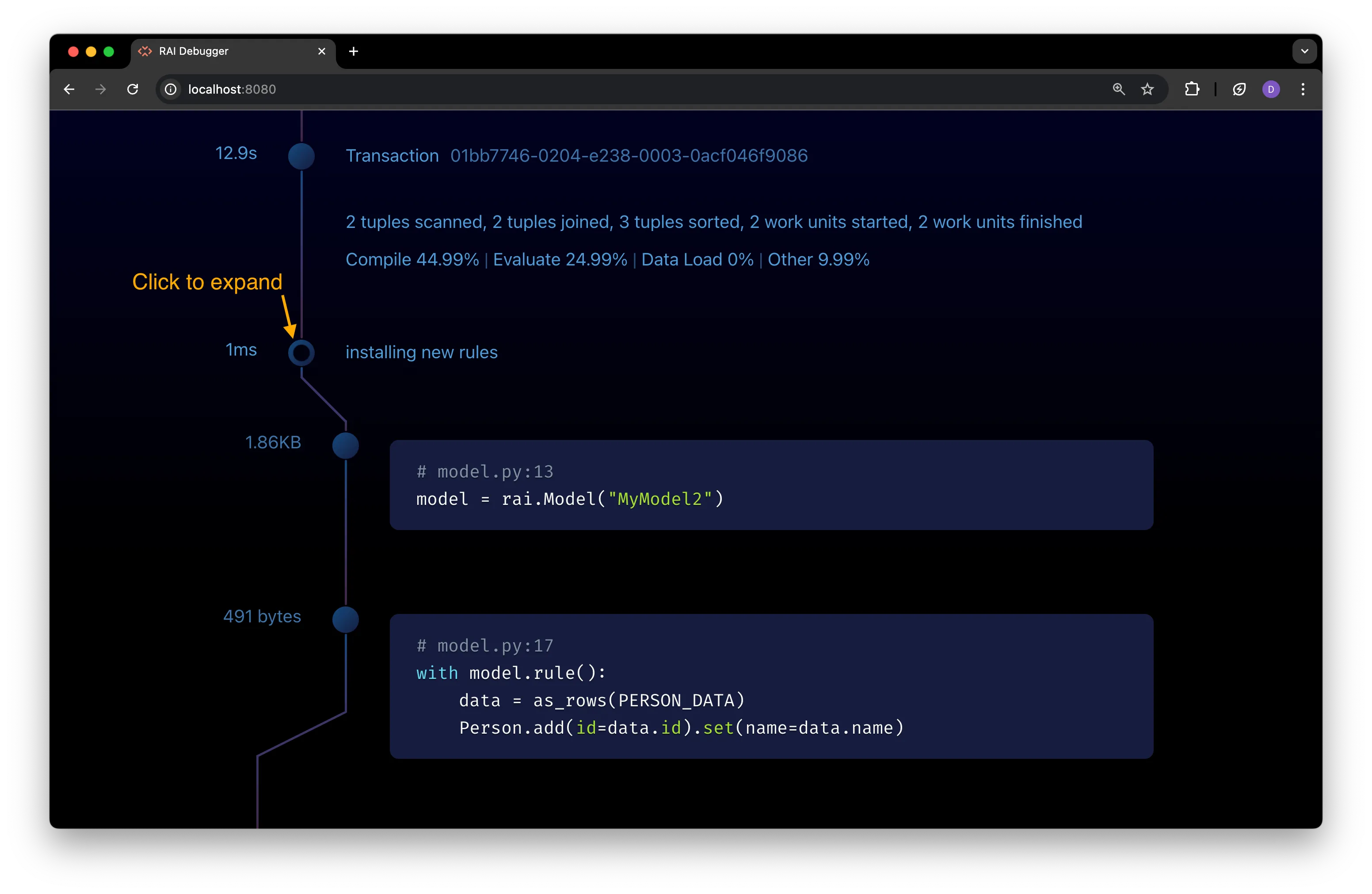
   Click on the rules node to open an expanded view with individual rules displayed in the timeline:

   

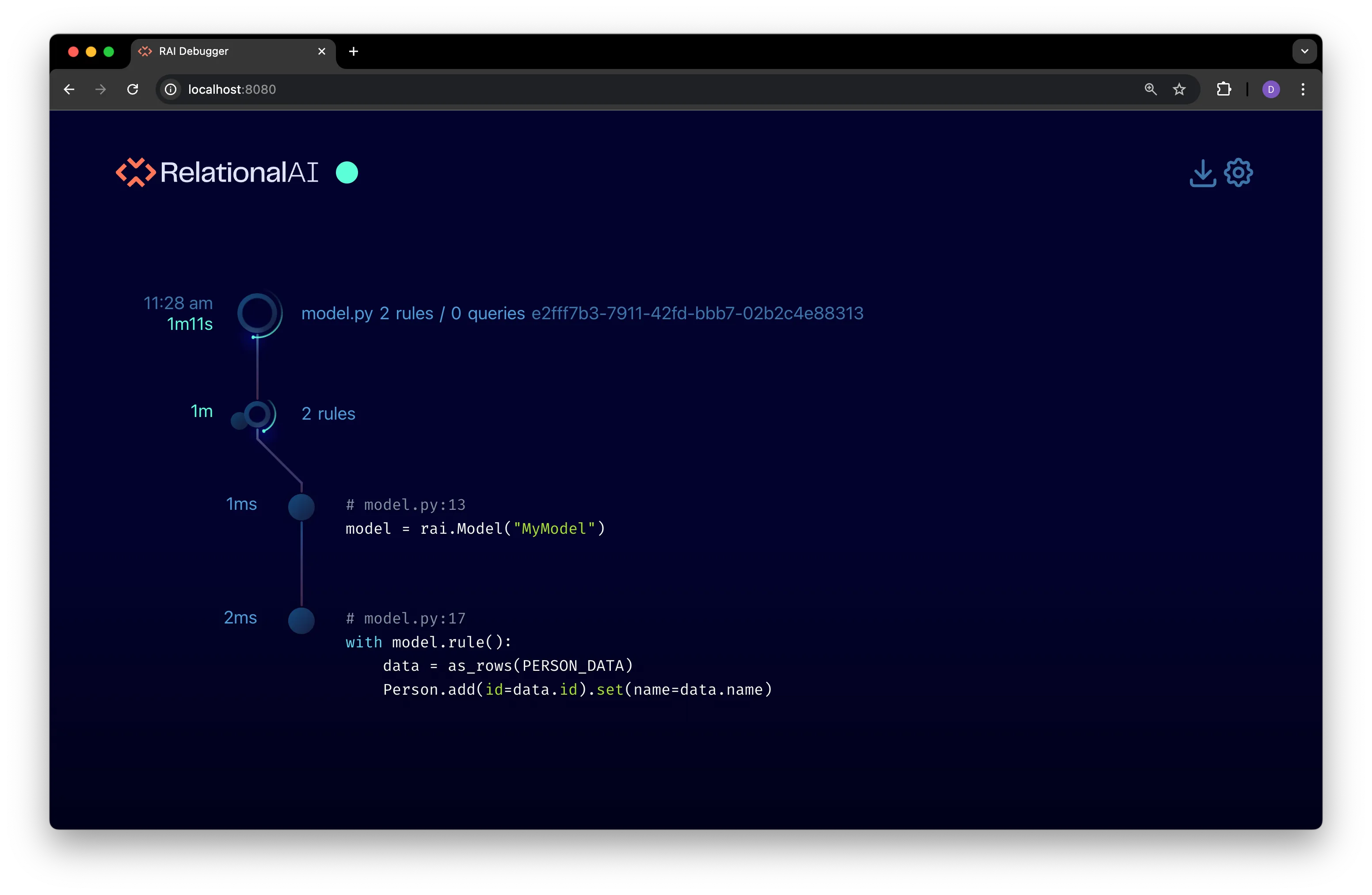
   This view updates as rules are compiled and installed in the model’s configured RAI engine. See Expanded Rules View for details on all the information available in this view.

   For now, click the rules node again to collapse it.

   Note

   Even though the my_project/model.py file has one model.rule() block, the timeline shows two rules. The Model constructor counts as a rule because, behind the scenes, it generates an initial batch of rules to set up the model.

   Other query-builder methods also generate rules without a model.rule() block, including Type.define() and Property.declare().

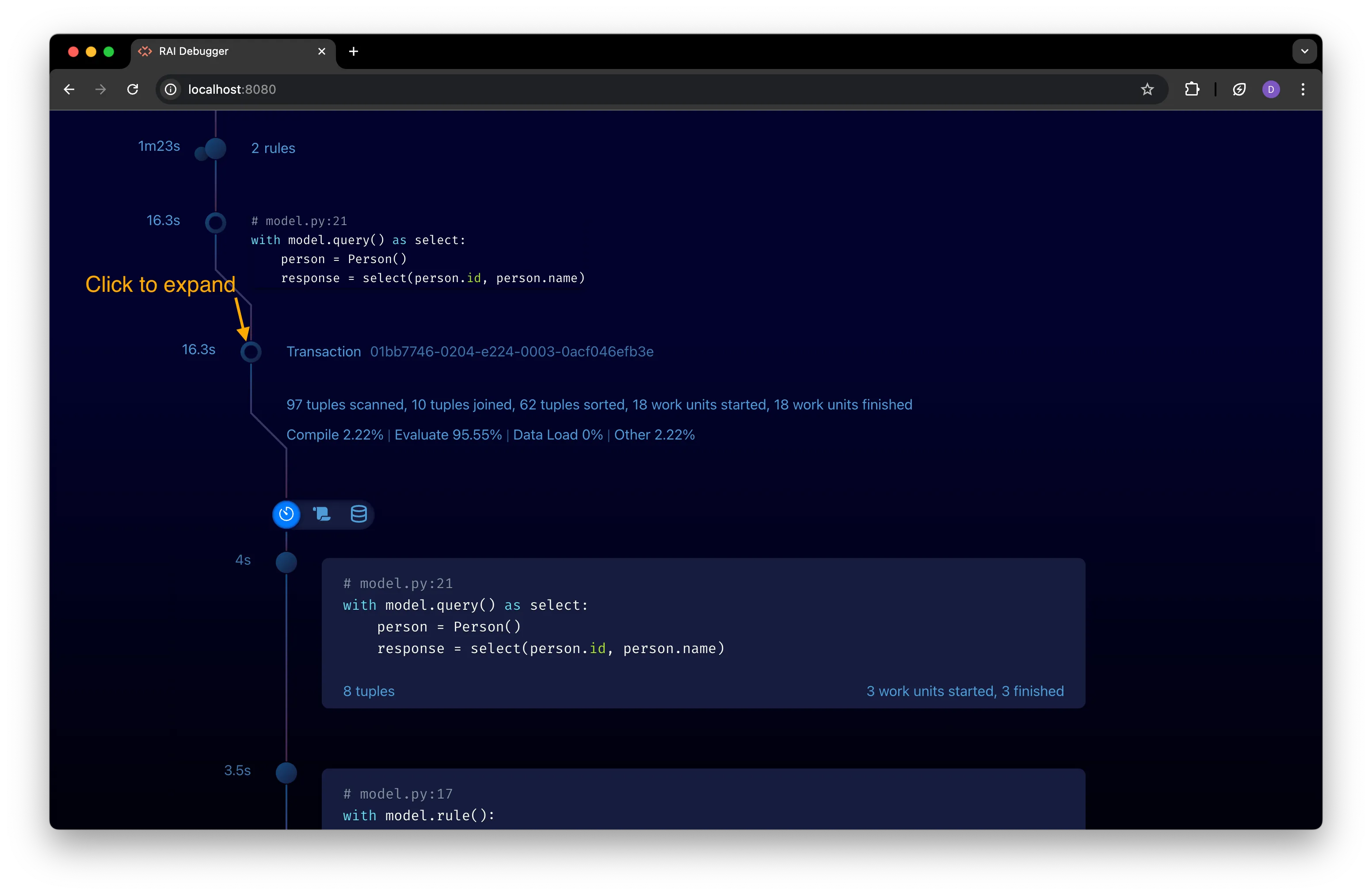
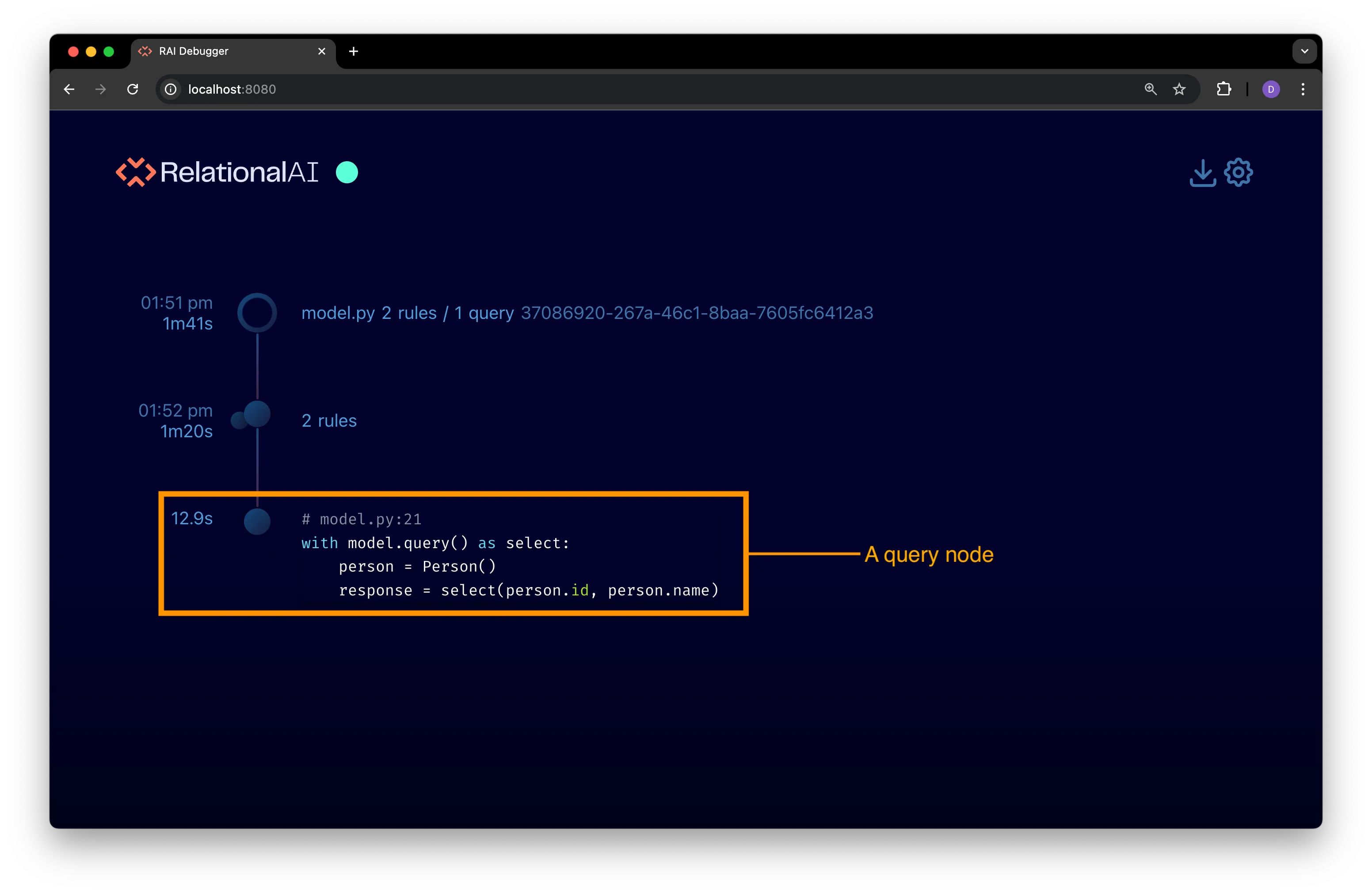
6. Explore the query node.

   Once the rules are compiled, a query node is created for the model.query() block in in the my_project/model.py file: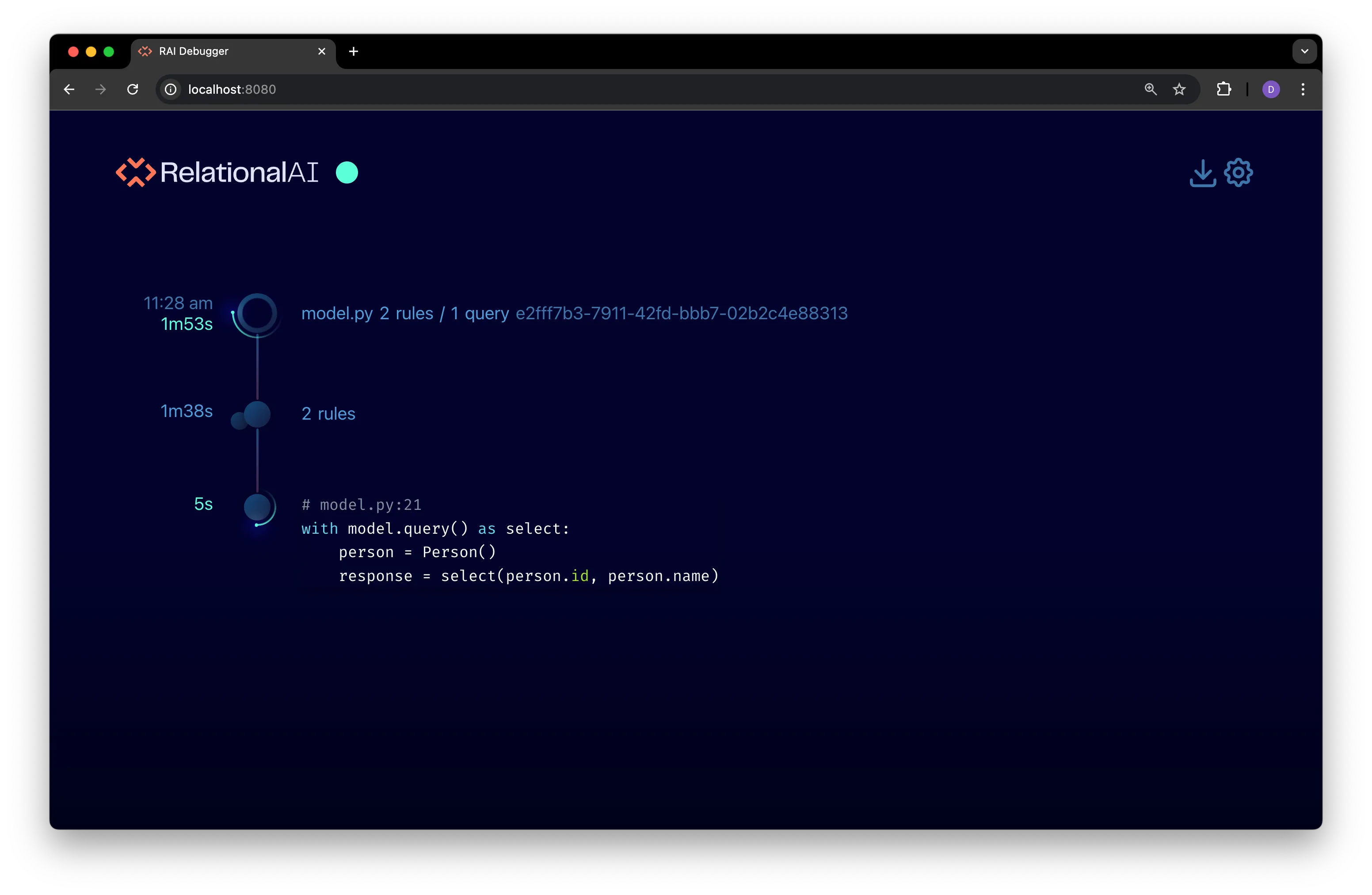

   

   You can view the query’s code and its elapsed execution time.

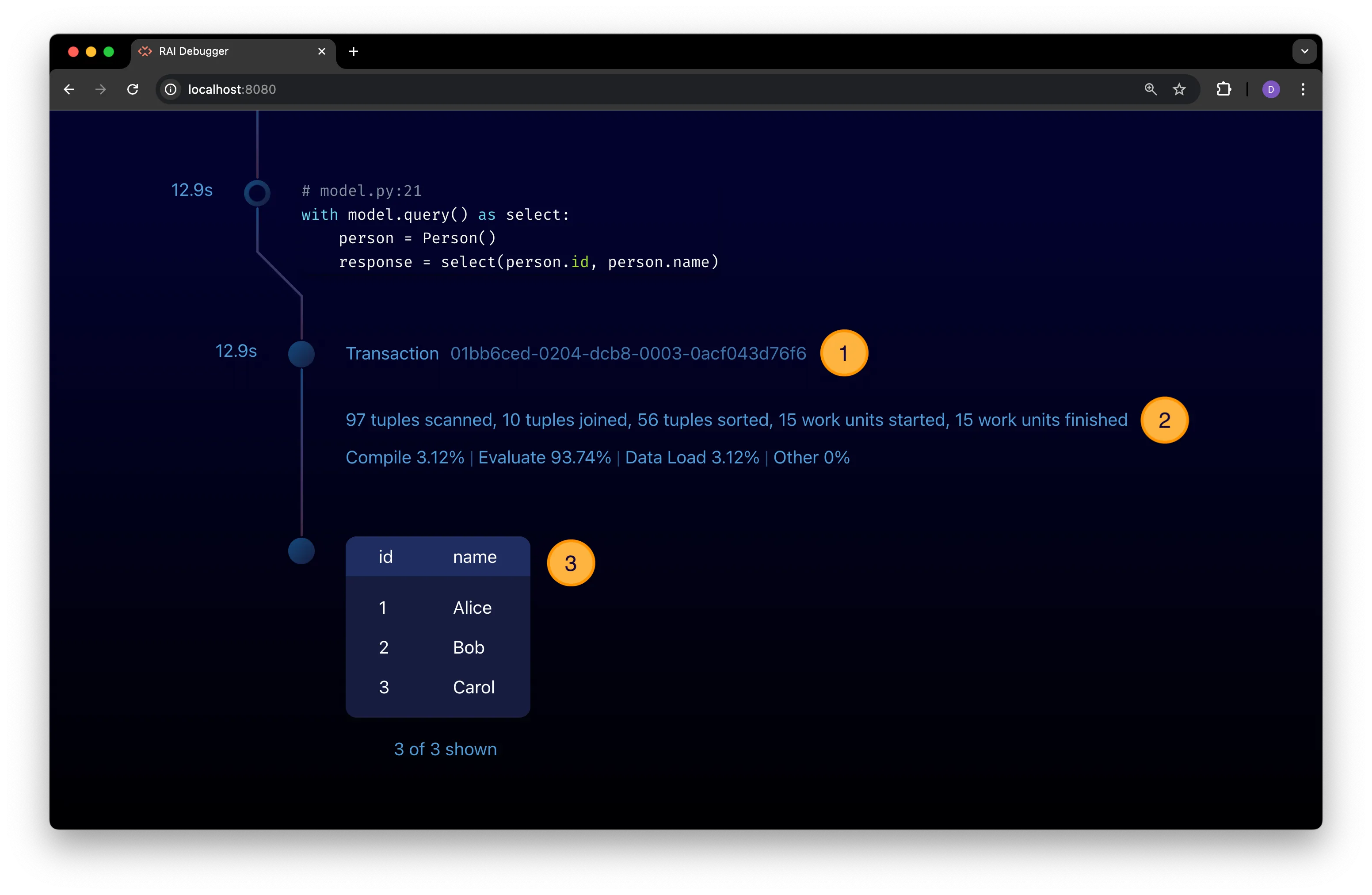
   Click on the query node for an expanded view that contains a transaction node with some basic profiling statistics for query:

   

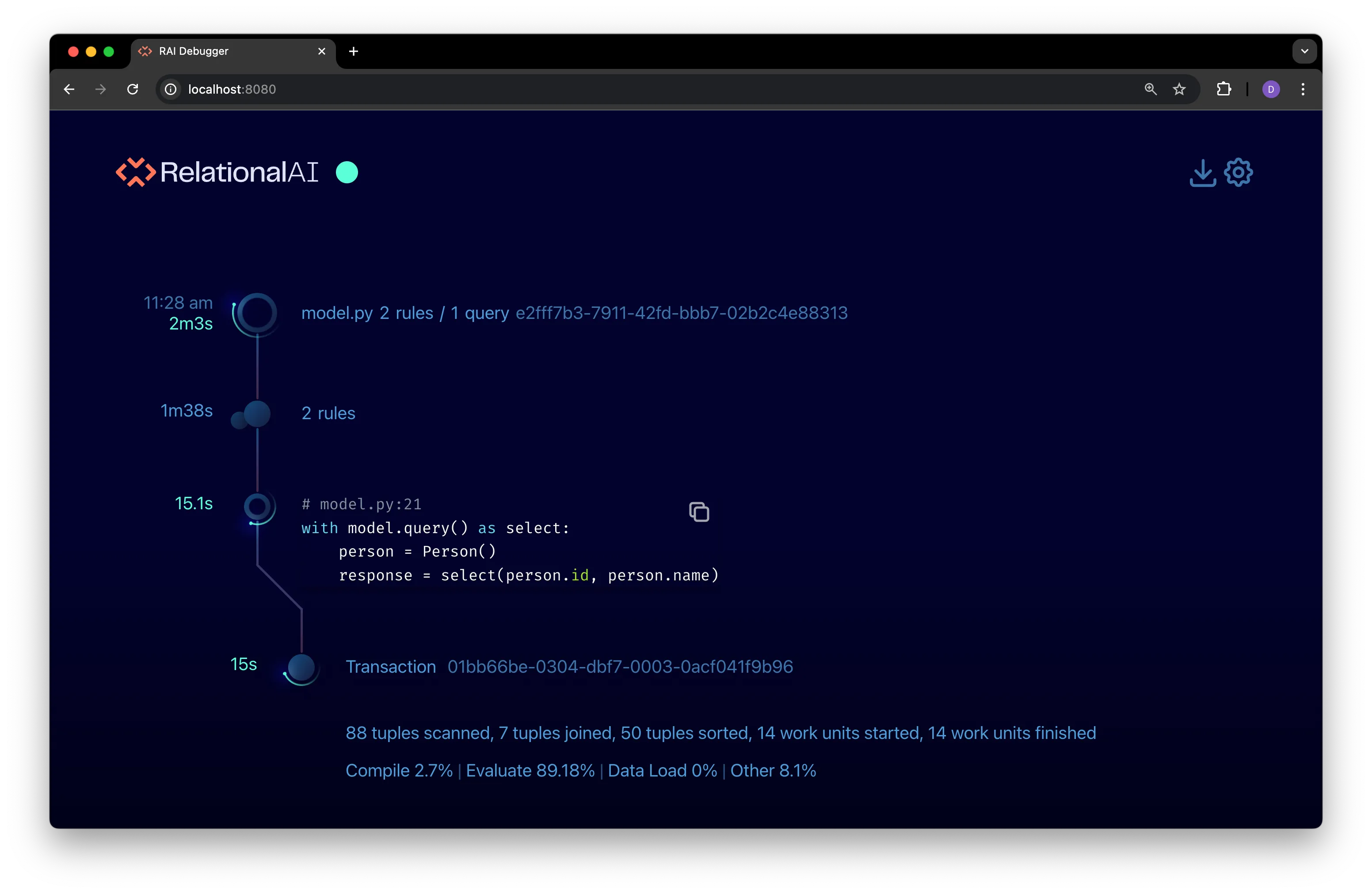
   Refer to Understand Profile Stats for details on interpreting these stats.

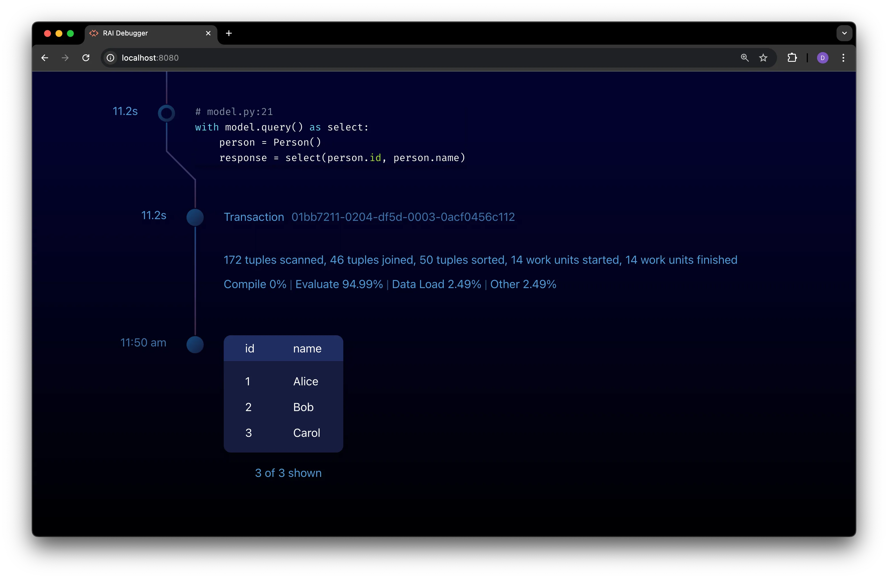
   When the query finishes, a sample of its results are displayed in the timeline:

   

View Error Information in the Debugger

If your program encounters an error, the debugger interface highlights the program node in orange and displays the error message in the timeline.

Follow these steps to run a program that generates an error:

1. Add new rules and queries to the program

   In the my_project/model.py file, add a new rule and query to the model:

   my_project/model.py

   import datetime
   
   import relationalai as rai
   from relationalai.std import as_rows, dates
   
   
   PERSON_DATA = [
      {"id": 1, "name": "Alice"},
      {"id": 2, "name": "Bob"},
      {"id": 3, "name": "Carol"},
   ]
   
   COMPANY_DATA = [                    # <-- Added new data
      {"id": 1, "name": "Acme", "date_founded": datetime.date(2019, 1, 1)},
      {"id": 2, "name": "Globex", "date_founded": datetime.date(2020, 2, 2)},
      {"id": 3, "name": "Initech", "date_founded": datetime.date(2021, 3, 3)},
   ]
   
   EMPLOYEE_DATA = [                   # <-- Added new data
      {"person_id": 1, "company_id": 1, "start_date": datetime.date(2019, 1, 1)},
      {"person_id": 2, "company_id": 1, "start_date": datetime.date(2020, 2, 2)},
      {"person_id": 3, "company_id": 2, "start_date": datetime.date(2021, 3, 3)},
   ]
   
   
   model = rai.Model("MyModel")
   Person = model.Type("Person")
   Company = model.Type("Company")                      # <-- Added new type
   Employee = model.Type("Employee")                    # <-- Added new type
   FoundingEmployee = model.Type("FoundingEmployee")    # <-- Added new type
   
   with model.rule():
      data = as_rows(PERSON_DATA)
      Person.add(id=data.id).set(name=data.name)
   
   with model.query() as select:
      person = Person()
      response = select(person.id, person.name)
   
   with model.rule():                                   # <-- Added new rule
      data = as_rows(COMPANY_DATA)
      Company.add(id=data.id).set(name=data.name)
   
   with model.rule():                                   # <-- Added new rule
      data = as_rows(EMPLOYEE_DATA)
      Employee.add(
         person_id=data.person_id,
         company_id=data.company_id
      ).set(start_date=data.start_date)
   
   # Define person and company properties for the Employees type that connect
   # employee entities directly to the person and company entities they are
   # related to.
   Employee.define(                                     # <-- Added new properties
      person=(Person, "id", "person_id"),
      company=(Company, "id", "company_id")
   )
   
   
   # An employee is a FoundingEmployee if they started working at the company
   # within 6 months of the company being founded.
   with model.rule():                                   # <-- Added new rule
      employee = Employee()
      company = Company()
      employee.start_date <= company.date_founded + dates.months(6)
      employee.set(FoundingEmployee)
   
   # Who are the founding employees?
   with model.query() as select:                        # <-- Added new query
      employee = FoundingEmployee()
      response = select(employee.person.name, employee.company.name)
   
   print(response.results)

2. Run the program.

   Save and run the edited model.py file:

   python model.py

   A new program node appears in the debugger interface:

   

   The second query in the new program encounters an error, which is indicated in the timeline by highlighting the query node in orange. The program node is also highlighted in orange to indicate that an error occurred during its execution:

   

   Note the order of events in the timeline:

   1. The program node is created.
   2. A rules node for 2 nodes is created.
   3. The first query is executed.
   4. A rules node with 3 nodes is created.
   5. The second query is executed, which causes an error.

   The program executes queries in the order that they appear in the code, and only the rules created before the query is executed are available to the query. The first query only uses the 2 rules created before it, while the second query uses all 8 rules.

   See The RAI Program Lifecycle for more details about the execution model.

3. View the error.

   Click on the highlighted query node’s timeline icon to view the error message:

   

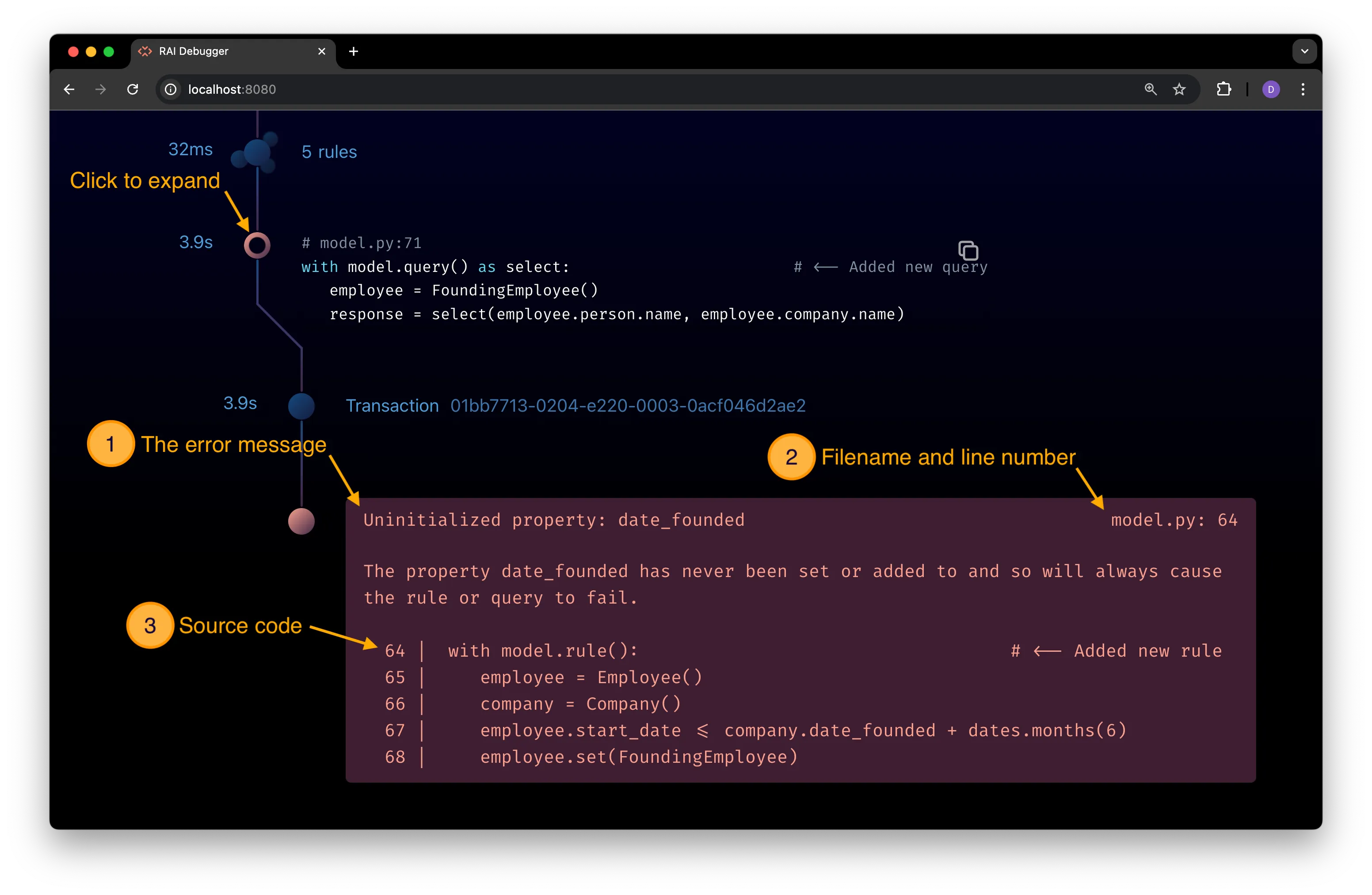
   The detailed view shows the following information about the error:

   1. The error message. In the preceding figure, the error message tells you that the date_founded property has never been set for Company entities.

   2. The filename and line number of the rule or query that generated the error. In the preceding figure, the error came from line 64 of the model.py file.

   3. The source code for the rule or query that generated the error. The code for the new query added to the program in Step 1 is displayed in the preceding figure.

4. Fix the error.

   The dictionaries in the COMPANY_DATA list defined at the top of the model.py file have a date_founded key with the date each company was founded:

   COMPANY_DATA = [
      {"id": 1, "name": "Acme", "date_founded": datetime.date(2019, 1, 1)},
      {"id": 2, "name": "Globex", "date_founded": datetime.date(2020, 2, 2)},
      {"id": 3, "name": "Initech", "date_founded": datetime.date(2021, 3, 3)},
   ]

   However, the rule defines Company entities from the data does not set a date_founded property:

   # Original rule
   
   with model.rule():
      data = as_rows(COMPANY_DATA)
      Company.add(id=data.id).set(name=data.name)  # <-- No date_founded property is set.

   To fix the error, edit the rule to set the date_founded property for Company entities:

   # Edited rule
   
   with model.rule():
      data = as_rows(COMPANY_DATA)
      Company.add(id=data.id).set(
         name=data.name,
         date_founded=data.date_founded # <-- Set date_founded property
      )

5. Re-run the program to check that the error is resolved.

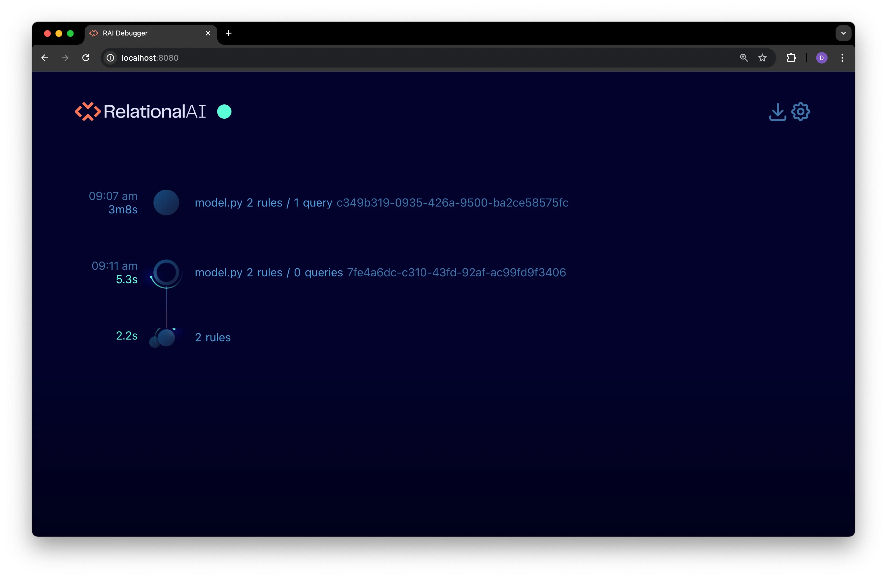
   Save and run the edited model.py file again. A third program node appears in the timeline. This time, the program completes without an error: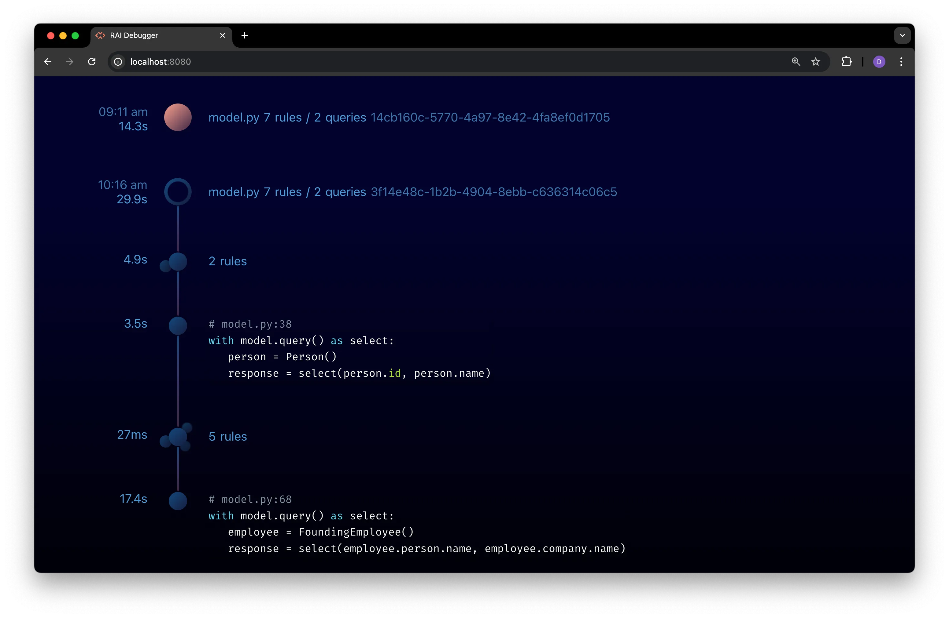

   

Debug a Query With Unexpected Results

Although the program completes without error, something still isn’t quite right.

1. Expand the query node to view query results.

   Click on the query node’s timeline icon to expand it and view the results of the query:

   

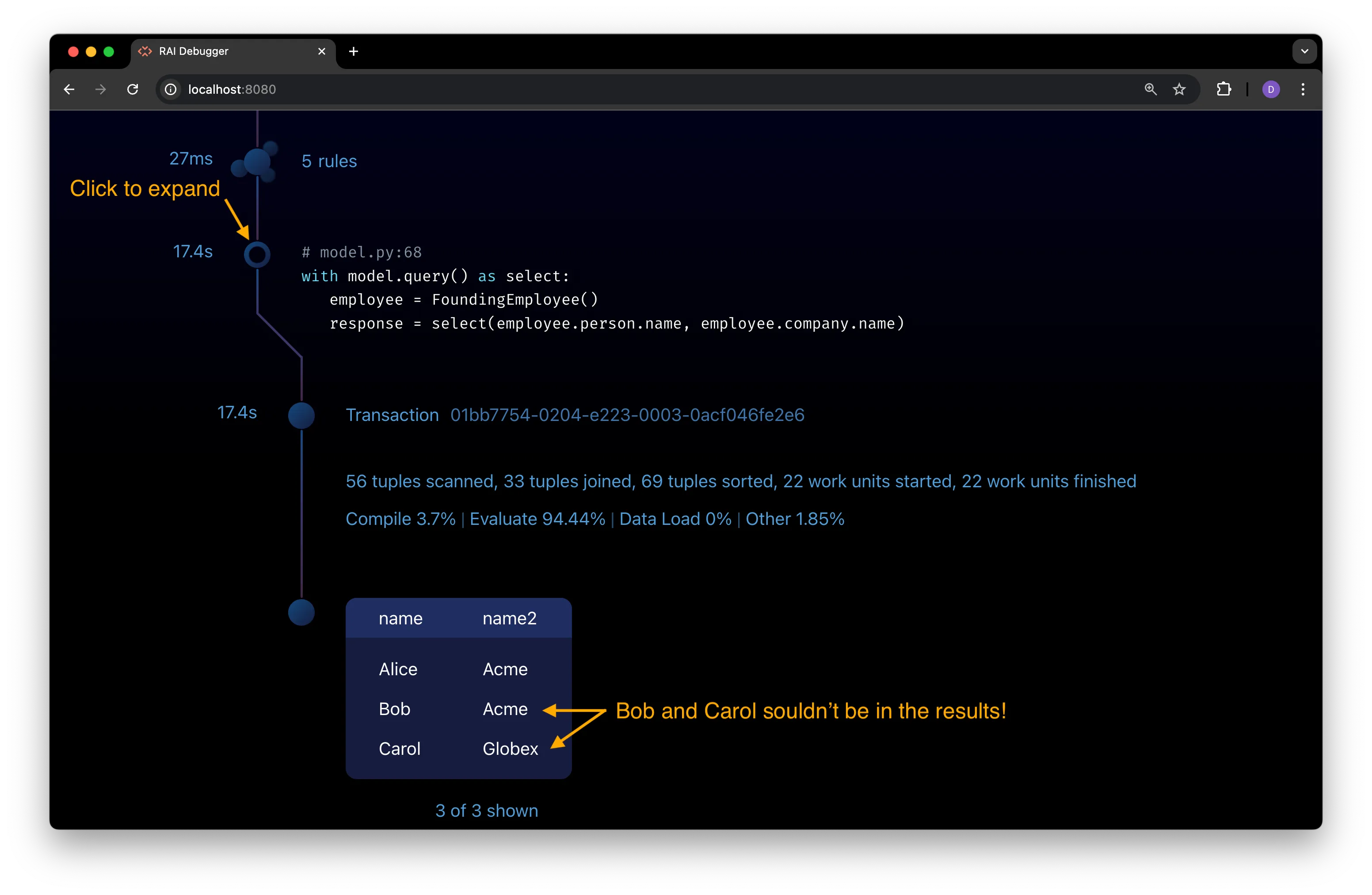
   The query returns the names of employees and companies where the employee is a founding employee of the company.

   According to the following rule, an employee is a founding employee if they started working at the company within 6 months of the company being founded:

   with model.rule():
      employee = Employee()
      company = Company()
      employee.start_date <= company.date_founded + dates.months(6)
      employee.set(FoundingEmployee)

   Bob isn’t a founding employee of Acme. He joined on February 2, 2021, over a year after the company was founded on January 1, 2020. In fact, Carol shouldn’t be a founding employee of Globex, either!

   Something is wrong with the rule, but what?

2. Expand the transaction node to view query execution details.

   Click on the transaction node to expand it:

   

   In the expanded view, you see each rule used to evaluate the query. Hover your mouse over a rule’s code to view all stats for the rule:

   

   See View Query Execution Details to learn how to interpret these stats.

3. Scan the rule blocks for issues.

   Scroll through the rules to see if any issues jump out to you.

   The rule that assigns Employee entities to the FoundingEmployee type has a warning icon in the bottom right corner: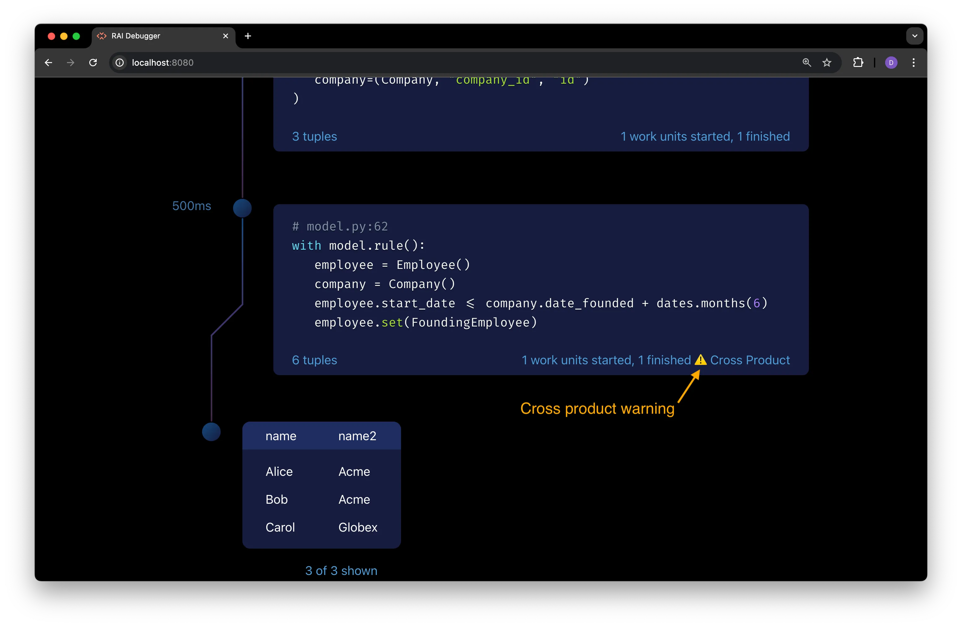

   

   This is a cross product warning. The employee and company variables have no constraint relating one to the other, so all possible pairs of employees and companies are being evaluated in the rule:

   with model.rule():
      employee = Employee()
      company = Company()  # <-- There is no condition that relates employee and company
      employee.start_date <= company.date_founded + dates.months(6)
      employee.set(FoundingEmployee)

   Bob gets paired with Globex, even though he doesn’t work there, and his start date is within 6 months of Globex’s founding date, so he is incorrectly assigned to the FoundingEmployee type.

4. Fix the cross product.

   Add a condition to the rule that relates the employee and company variables:

   with model.rule():
      employee = Employee()
      company = Company()
      employee.company_id == company.id  # <-- Add condition to relate employee and company
      employee.start_date <= company.date_founded + dates.months(6)
      employee.set(FoundingEmployee)

   Alternatively, you can reference the employee’s company property directly:

   with model.rule():                      #  Get employee's company property
      employee = Employee()                # /
      #                      ∨∨∨∨∨∨∨∨∨∨∨∨∨∨∨∨
      employee.start_data <= employee.company.date_founded + dates.months(6)
      employee.set(FoundingEmployee)

   See Interpret Cross Product Warnings for more details about cross products and how to fix them.

5. Re-run the program to check that the query works as expected.

   Save and run the edited model.py file again. The query now returns the expected results: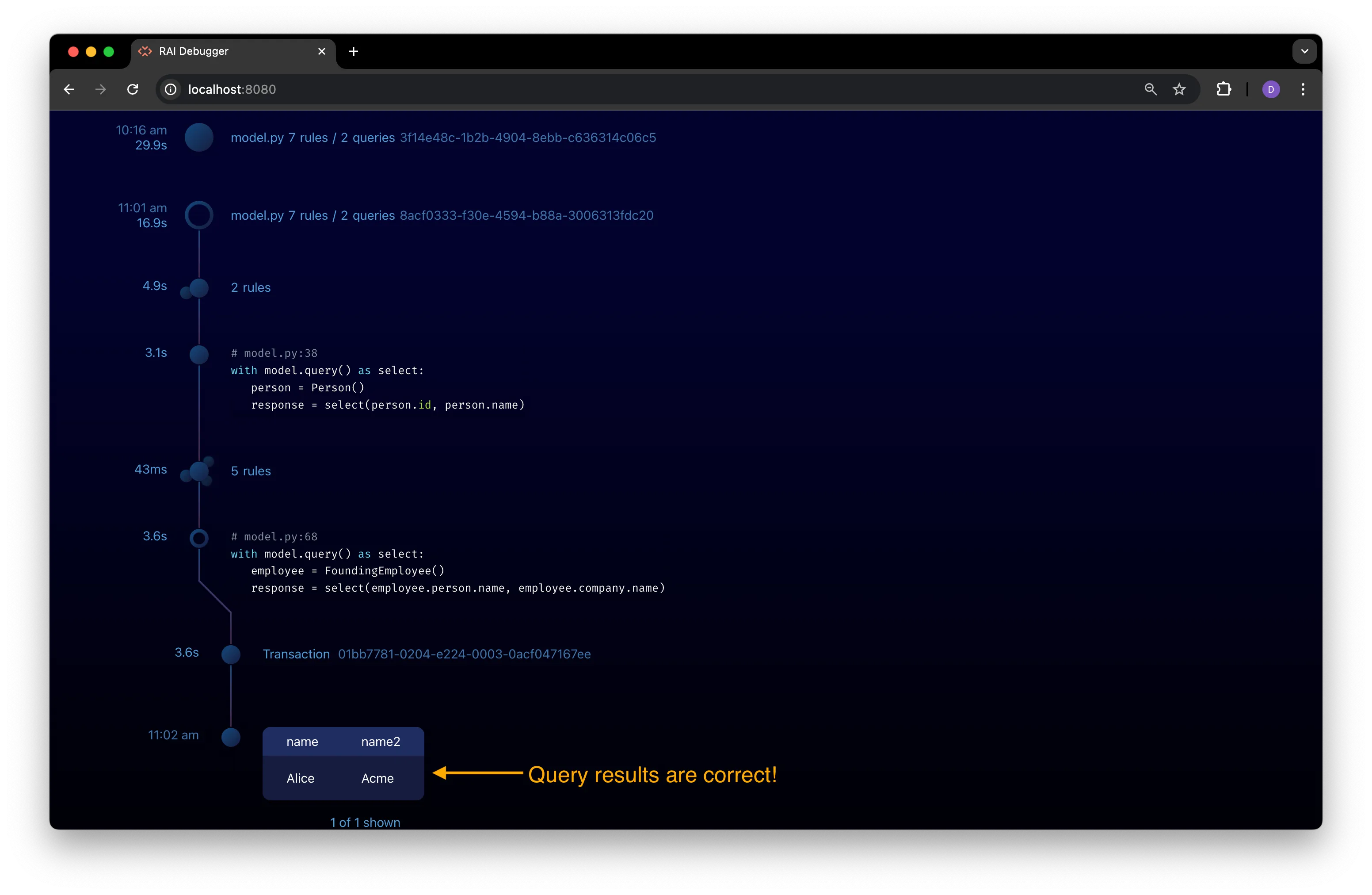

   

Export Detailed Debugger Logs

If necessary, you can export events logged by the debugger to share with RelationalAI support or to send to someone else to help debug your program.

Note

By default, debugger logs are stripped of sensitive information, including query results. This may be modified in the Settings window by toggling the Strip sensitive data on export option on or off.

To export a log file, scroll to the very top of the debugger interface in your browser and click on the Export events button in the top right corner to the left of the gear icon:

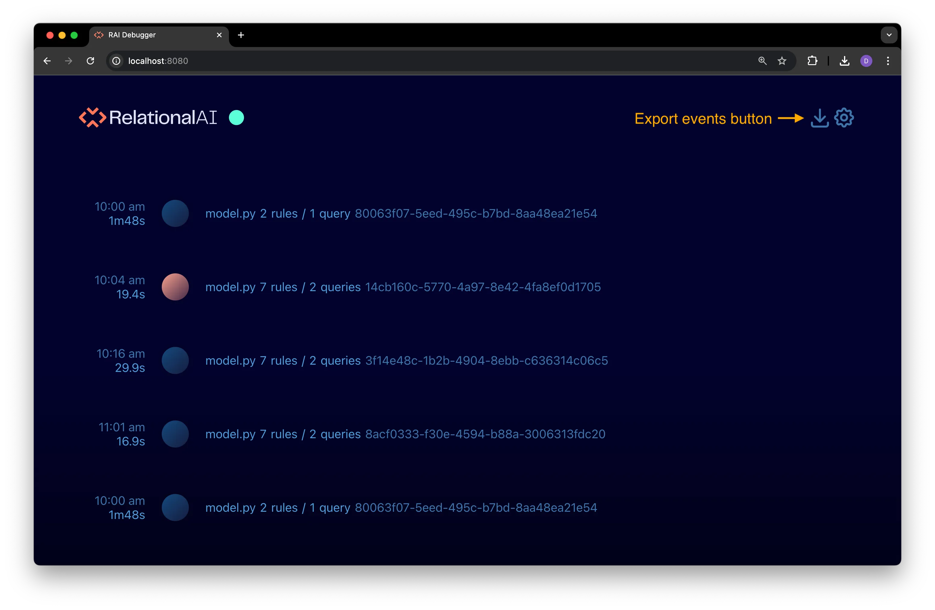
The file is saved as debugger_data.json to the same directory where you started the debugger server. You can open the file in a text editor or JSON viewer to see the raw log data. , and may share the file with others.

Load an Exported Log File

To view an exported debugger log, drag and drop the debugger_data.json file onto the debugger interface. The debugger timeline is cleared and the contents of the file are rendered in the interface as a new timeline.

Use the Debugger With a Jupyter Notebook

The debugger can be used to view programs run in Jupyter notebooks. After you’ve started the debug server, you can start a Jupyter notebook server in a separate terminal window and execute cells from a notebook.

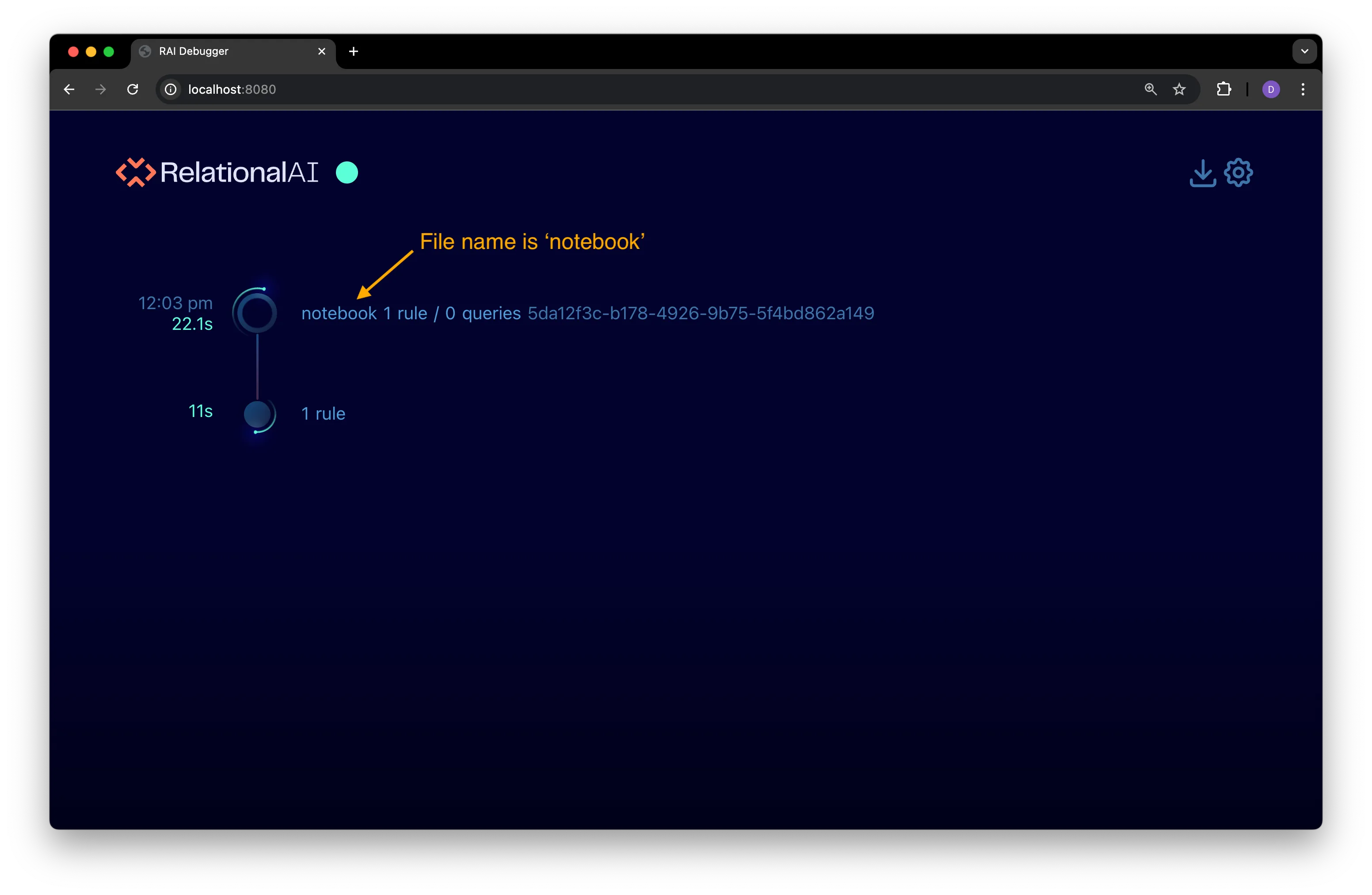
The timeline for the notebook is displayed in the debugger interface:

Note that:

• A program node only appears when a cell calls the Model constructor. Until that cell is executed, the debugger timeline might be empty.

• The file name displayed with the program node is notebook (see preceding figure).

• The program node is shown as running—indicated by a bright green spinner around its timeline icon like the preceding figure—as long as the Jupyter kernel is running.

• Restarting the Jupyter kernel and re-running the notebook creates a new program node in the timeline.

Tip

Executing cells out of order can lead to inconsistent rules and unexpected behavior that may be difficult to debug.

Sometimes, resetting the notebook’s state by restarting the kernel and re-running all cells can resolve issues.

Understand the Debugger Interface

The RAI debugger displays events logged during a program’s execution as a timeline in a web browser window. The timeline has several different components, including:

• A main menu with buttons to export events, clear the timeline, and open the settings panel.
• Program nodes that represent the execution of a program and expand to show a detailed timeline of the program’s execution.
• Rules nodes that represent the compilation of rules in the program and expand to show details about the rules.
• Query nodes that represent the execution of queries in the program and expand to show details about the query execution.
• Transaction nodes that represent the execution a transaction on a RAI engine and provide profiling statistics for the transaction.

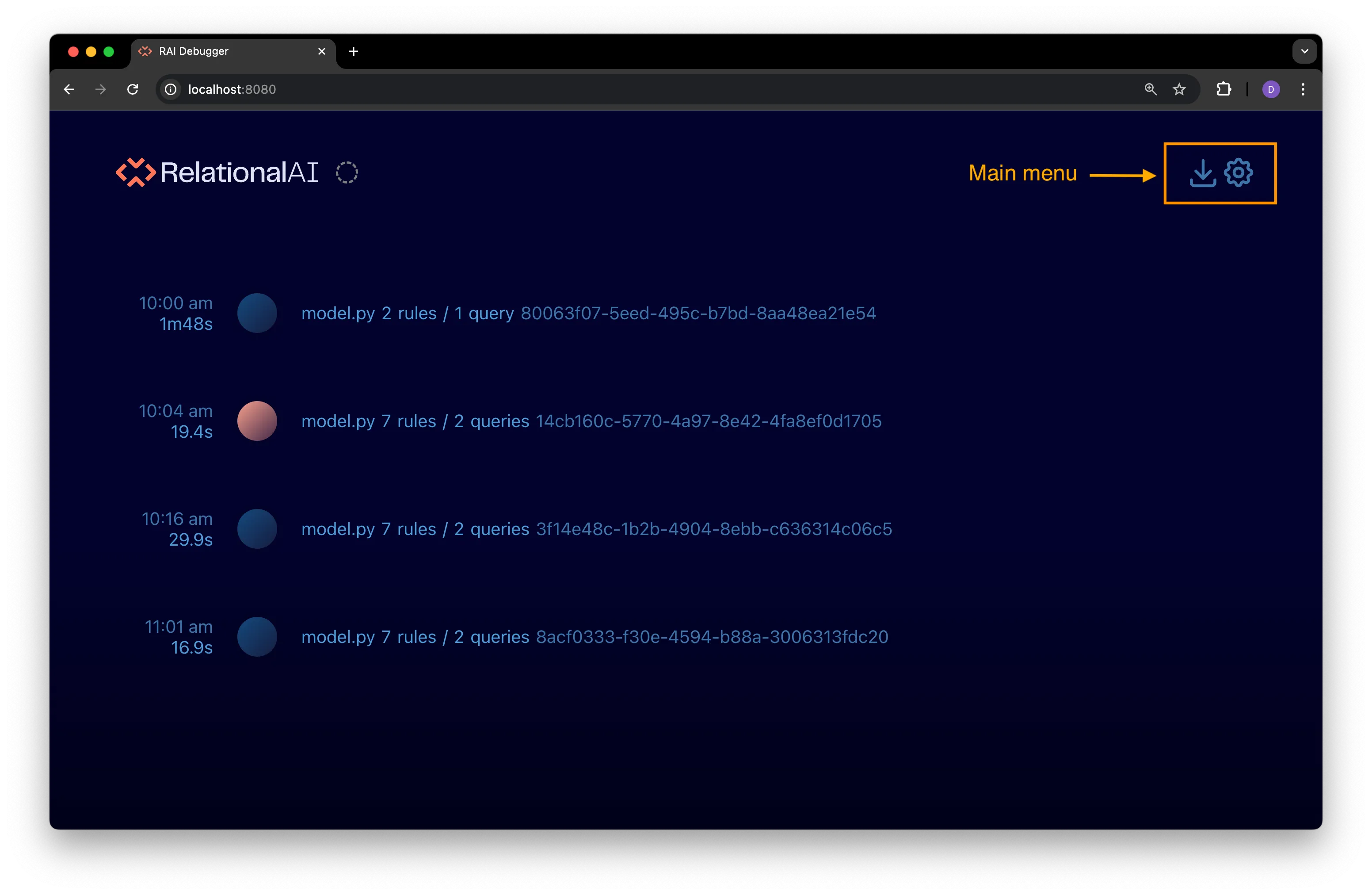
Main Menu

The main menu is located in the top right-hand corner of the debugger interface:

Tip

If you can’t see the main menu, you may need to scroll to the top of the debugger window to see it

Hovering over the main menu exposes the following buttons:

• Settings
• Export Events
• Follow Last Run
• Clear Events

Settings Button

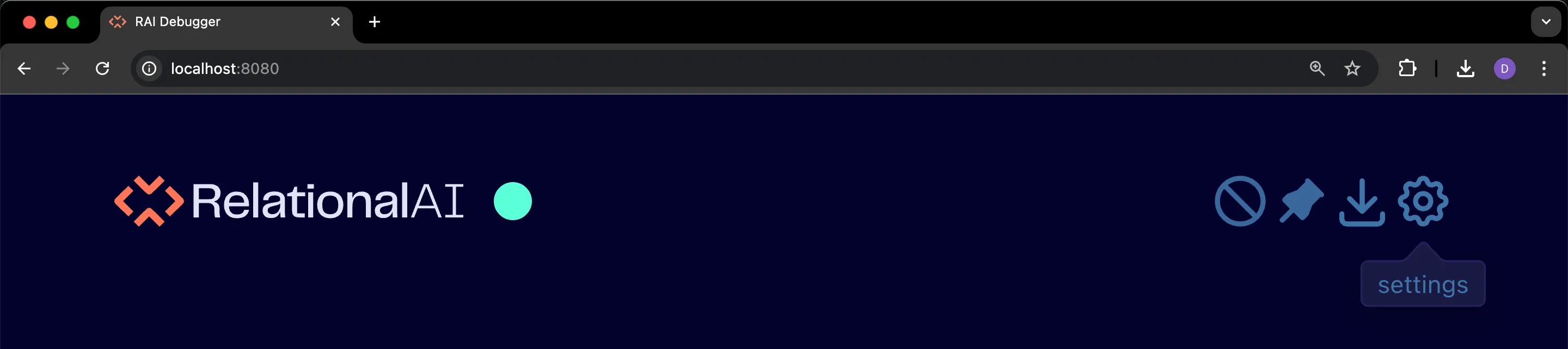
Click on the settings button to open the settings panel:

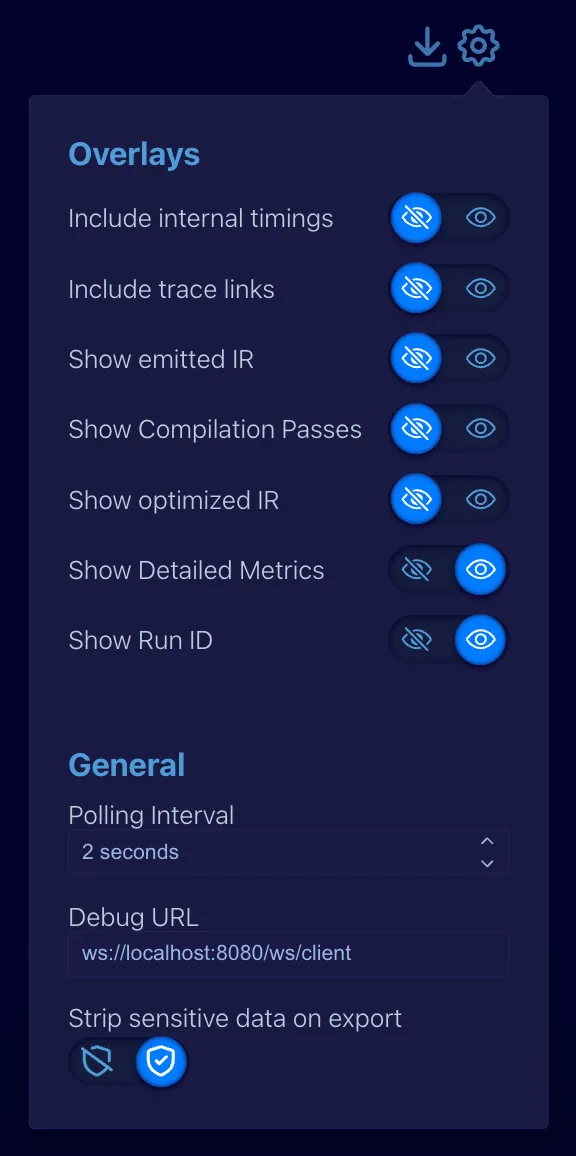
This panel has switches to enable or disable a number or options. The recommended settings are shown in the preceding figure, with everything disabled except for the Show Run ID options. Most other options are meant for internal use by RelationalAI support.

The Overlay options allow you to toggle between more or less detailed views of the timeline. Bolded settings in the table below are the recommended settings for most users:

Option	Description	Default
Include internal timings	When enabled, the timeline includes timing information for internal operations. Intended for RAI support use only.	Disabled
Include trace links	When enabled, shows trace links in the timeline. Intended for RAI support use only.	Disabled
Show emitted IR	When enabled, shows compiled IR for rules and queries. Intended for RAI support use only.	Disabled
Show compilation passes	When enabled, includes detailed compilation information. Intended for RAI support use only.	Disabled
Show optimized IR	When enabled, shows additional information about the compiled IR. Intended for RAI support use only.	Disabled
Show Detailed Metrics	When enabled, shows detailed information and profile stats for rules and queries. Intended for RAI support use only.	Disabled
Show Run ID	When enabled, shows the unique Run ID for the program.	Enabled

General options include:

Option	Description	Default
Polling interval	The interval in seconds at which the debugger checks for new events.	2 seconds
Debug URL	The debug server URL.	ws://localhost:8080/ws/client
Strip sensitive data on export	When enabled (shield with check mark icon), sensitive data is removed from the log file exported when you click the Export events button so that logs are safe to share with RAI support.	Enabled

Export Events Button

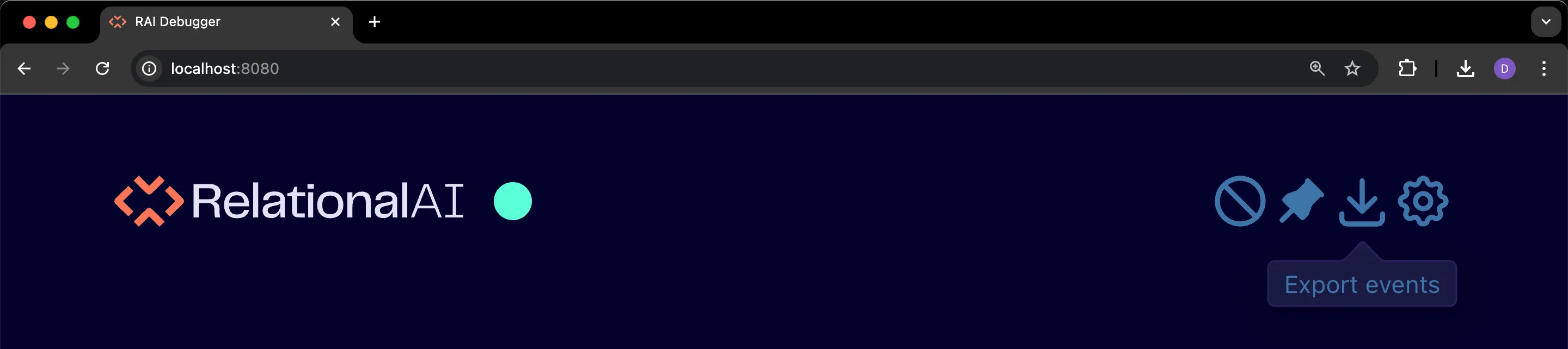
Click the Export events button to export a file named debugger_data.json with all of the events logged by the debugger. See Export Detailed Debugger Logs for details.

Follow Last Run Button

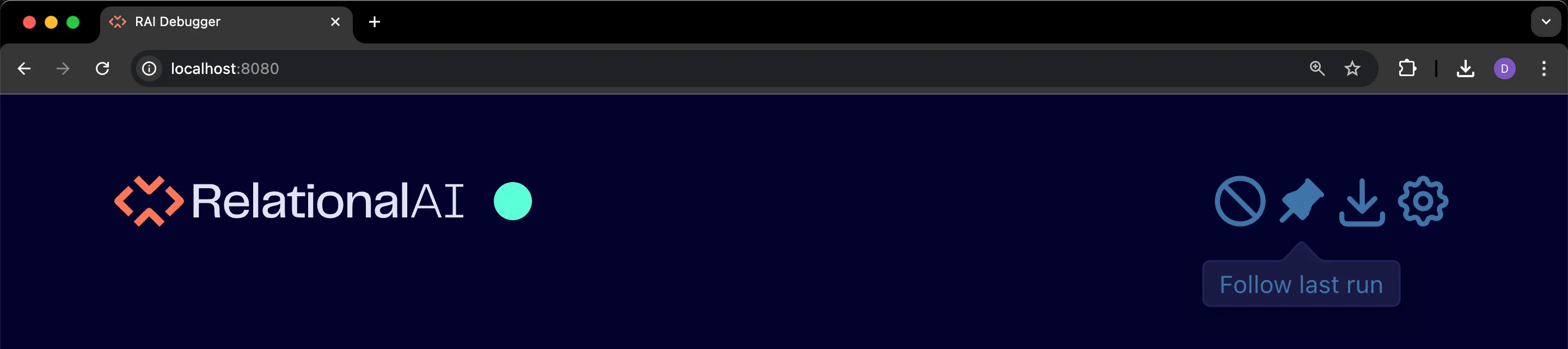
Click the Follow last run button to ensure that the most recent run is always expanded in the timeline.

Clear Events Button

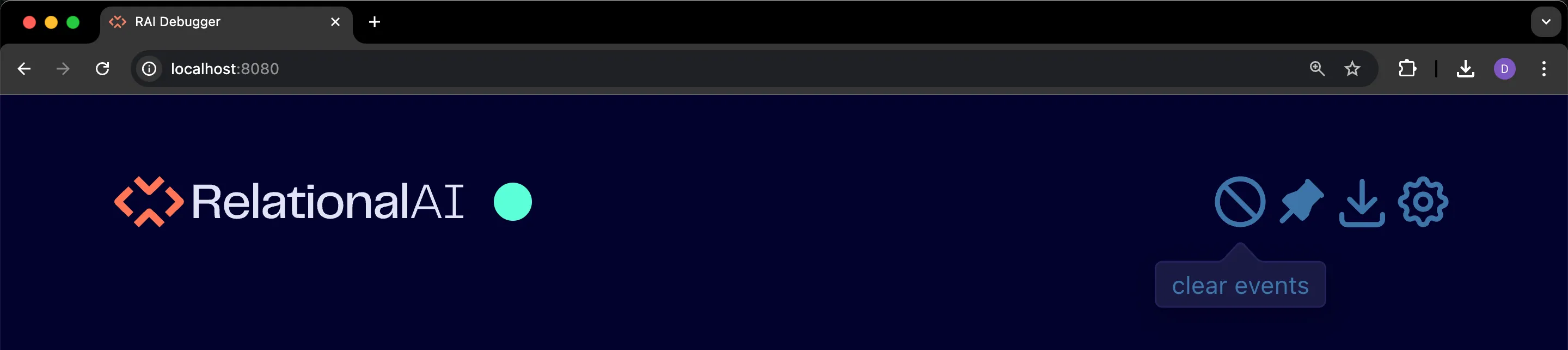
Click the Clear events button to clear the debugger timeline.

Program Nodes

Program nodes are shown on the execution timeline with a large dot icon:

Compact Program View

In the default compact view, the program node shows:

• The timestamp when the program started executing.
• The elapsed time for the program to execute.
• The number of rules and queries that have been compiled during the program’s execution.
• The unique Run ID for the program.

A program node highlighted in orange indicates that an error occurred during the program’s execution. See View Error Information in the Debugger to learn how to view error messages.

Expanded Program View

Click on a program node’s timeline icon for an expanded view with all of the rules nodes and query nodes associated with the program’s execution:

Rules Nodes

Rules are shown on the execution timeline with an icon that looks like multiple dots. In the following example, the timeline has two rules that have been compiled:

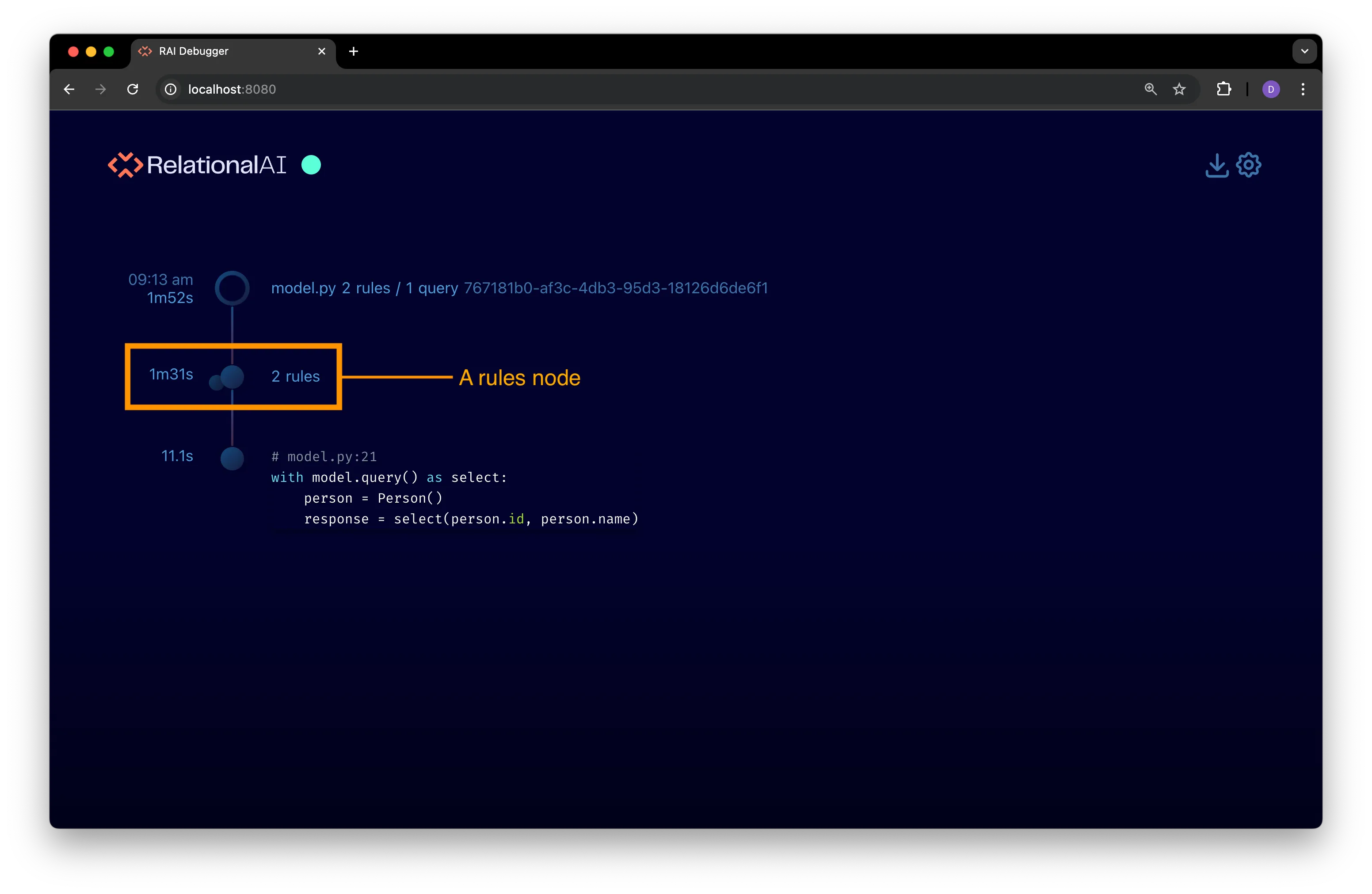
Compact Rules View

You can view the following information in the default compact node view:

• The total compilation time for the rules to the left of the node.
• The number of rules that have been compiled to the right of the node.

Note

The “total compilation time” may include time spent on other tasks, such as preparing data sources or creating your RAI engine.

Expanded Rules View

Click the dot next to a rules node to expand it and view details about the rules that have been compiled:

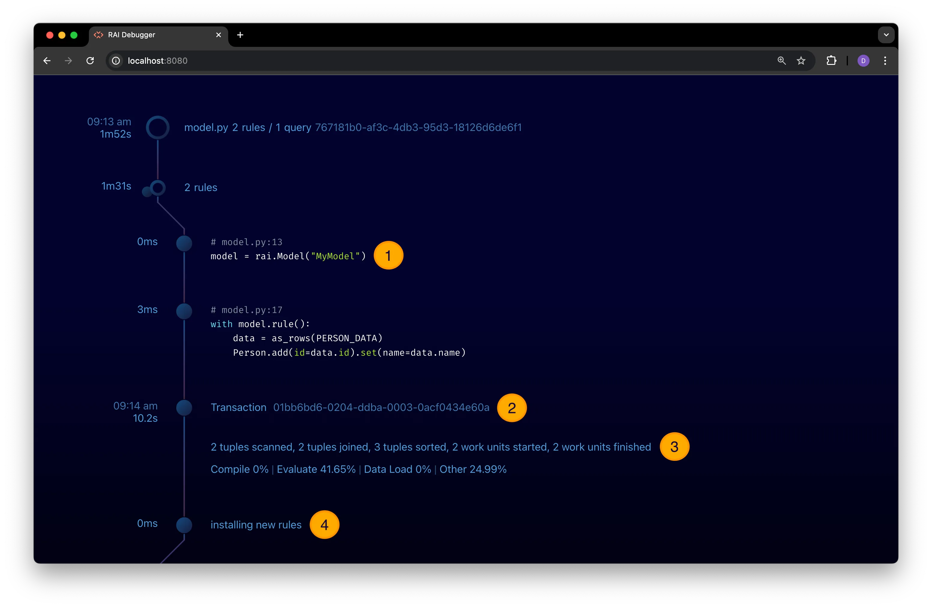
The expanded view shows:

1. The code for each rule along with its compilation time and the filename and line number where the rule was defined.

   Tip

   Hover your mouse over a rule’s code and click the copy button in the top right corner to copy a rule’s code to your clipboard:

   

2. A transaction node with the total elapsed transaction time and the transaction’s unique ID.

3. Several profile statistics for the transaction’s execution. See Understand Profile Stats to learn how to interpret these stats.

4. An installation node that can be expanded to view details about the compiled rules. See View Rule Compilation Details for details.

Query Nodes

Query nodes are shown on the execution timeline as a single dot with the query’s code next to it:

Compact Query View

With the default compact node view (see preceding figure) you can see:

• The total elapsed query execution time.
• The query’s code and the filename and line number where the query was defined.

Expanded Query View

Click on a query node for an expanded node view with details about the query and its execution:

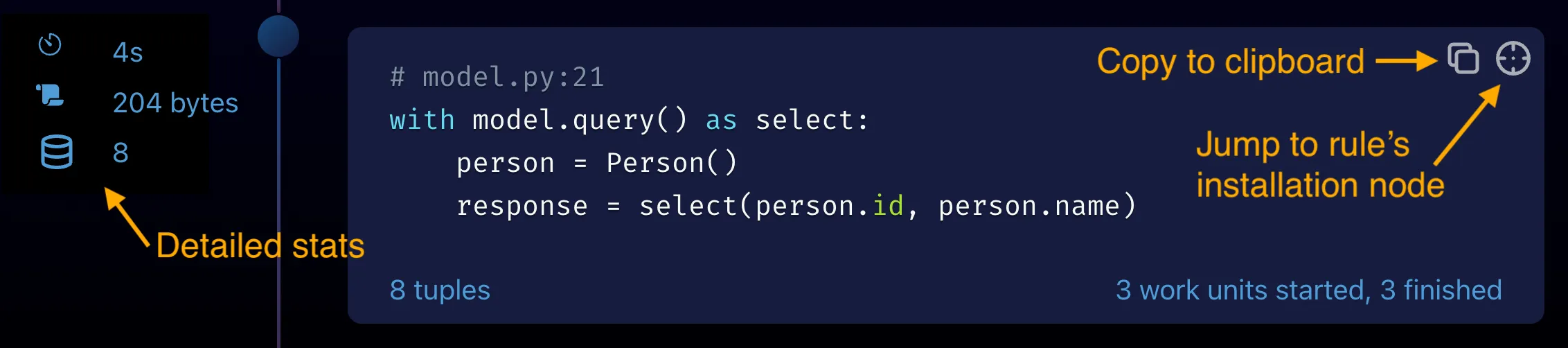
The expanded view shows:

1. A transaction node with the transaction’s unique ID and its total elapsed execution time.

2. Some profiling statistics for the query execution including tuple and execution stats. See Understand Profile Stats for more details on these stats.

   Tip

   Click on the dot next to the transaction node to expand it and view detailed profile information for the query execution. See View Query Execution Details for more information.

3. A table with the query results.

Transaction Nodes

Transaction nodes are shown on the execution timeline as a single dot labeled with the word Transaction and a unique ID:

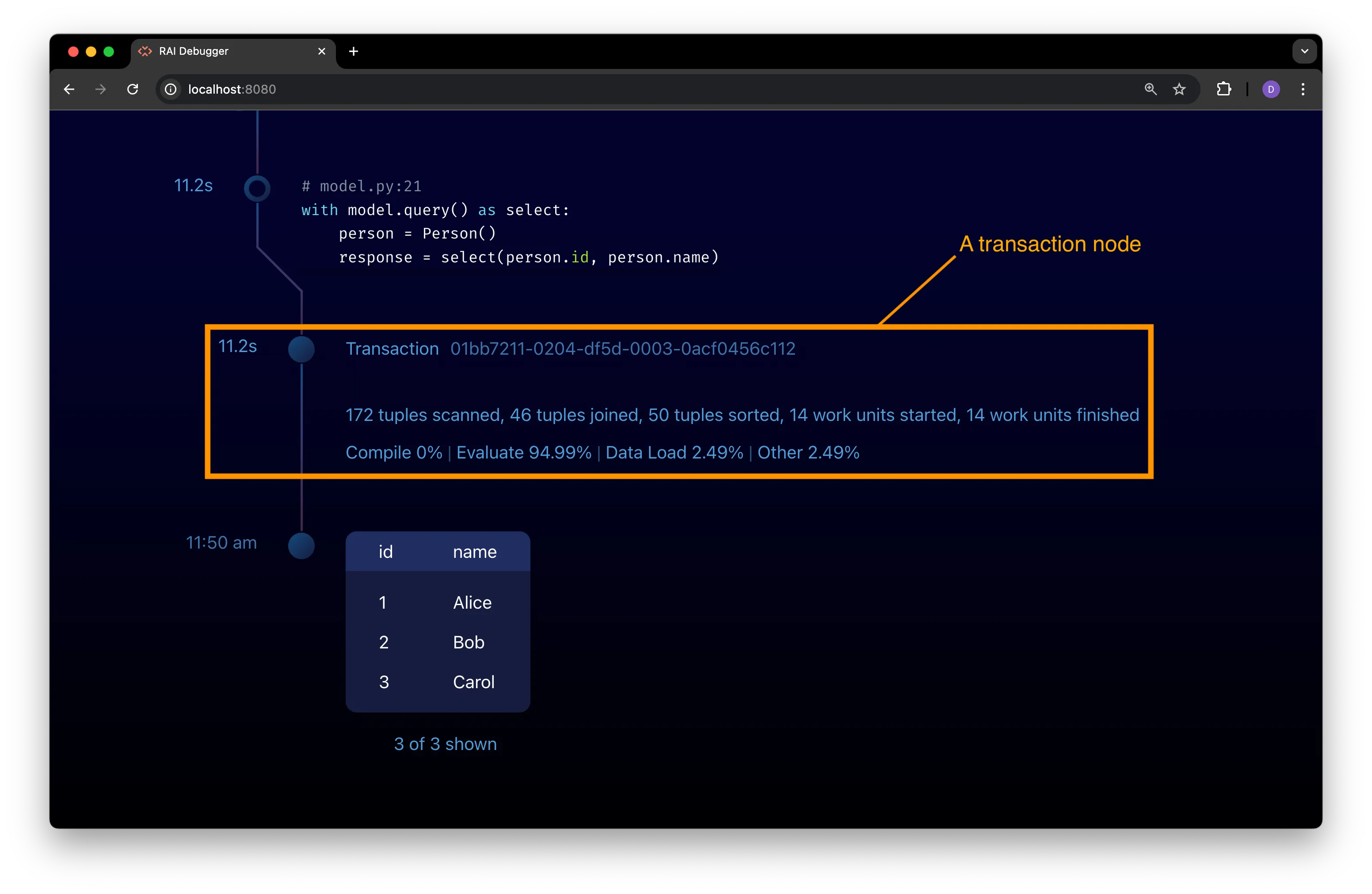
Both rules nodes and query nodes may have a transaction node in their expanded view.

Below the transaction node is some basic profiling statistics for the transaction. See Understand Profile Stats for details on interpreting these statistics.

Note

You can also view transaction information using the transactions:get CLI command or the get_transaction() SQL procedure.

Profile stats are only available in the debugger interface.

The debug.jsonl File

When you run a program with the debugger enabled, a debug.jsonl file is created in the directory that you ran the program from. This file contains the raw debug logs for the most recent program execution, since each time you run the program the file is overwritten.

You can view the contents of the debug.jsonl file using the debugger interface by dragging and dropping the file into your browser window with the debugger open. Note that the timeline in the debugger interface is cleared and the contents of the debug.jsonl file are rendered as a new timeline.

Tip

You can save your current timeline before loading a debug.jsonl file. See Export Detailed Debugger Logs for details.

Multiple Connections

The debug server can accept a connection from any program running on a machine with access to the server’s network URL. You can view the URL in the settings panel.

Multiple programs can be viewed in the same timeline. Each program is represented by its own program node.

Understand Profile Stats

The profile statistics displayed by transaction nodes expose information about the execution of a transaction. To fully understand the profile stats, it helps to understand the execution model for a RAI program.

The RAI Program Lifecycle

When you query a model built with the RAI Python API, the query is not evaluated on your local machine. The model sends transactions to the RAI engine specified in the model’s configuration. The engine evaluates the query and results are returned to the local Python runtime.

Query Execution Loop

Programs execute in a loop that repeats the following three steps:

1. Collect rules.

   Each rule context encountered by the interpreter generates logic in an intermediate representation (IR) that is tracked by the program’s Model object. The model collects rules until the interpreter encounters a query context.

2. Install compiled rules.

   When the first query context is interpreted, all of the rules collected in Step 1 are compiled together. A transaction is sent to the model’s RAI engine to install the compiled IR so that this and all subsequent queries can use the rules without recompiling them.

3. Evaluate a query.

   The logic contained in a query context is compiled into IR and sent to the engine for evaluation in another transaction. Your local Python runtime blocks until results are returned.

   Once a transaction returns query results, the local runtime continues to interpret your program by returning to Step 1 to process more rules until the next query context is encountered.

Note

Programs are executed statelessly, meaning the RAI engine doesn’t cache any data between program executions. This includes rules compiled by the model and any data generated to evaluate queries. The next time a program is run, everything starts from scratch.

The only exception is if you run the exact same program two or more times consecutively. RAI engines cache the results of transactions. When a transaction is identical to the one prior to it, the cached results are used instead of re-evaluating the transaction.

Execution Phases

Transaction execution is divided into multiple execution phases:

• During the compilation phase, a query plan is generated for the transaction.
• The query plan is evaluated during the evaluation phase.
• Any data that must be loaded for the transaction is done during a data load phase.

The percentage of total time spent in each of these phases is shown in the compact stats view displayed below the transaction node.

Read Compact Profile Stats

A transaction node’s default compact view displays statistics that give an overview of the transaction’s execution:

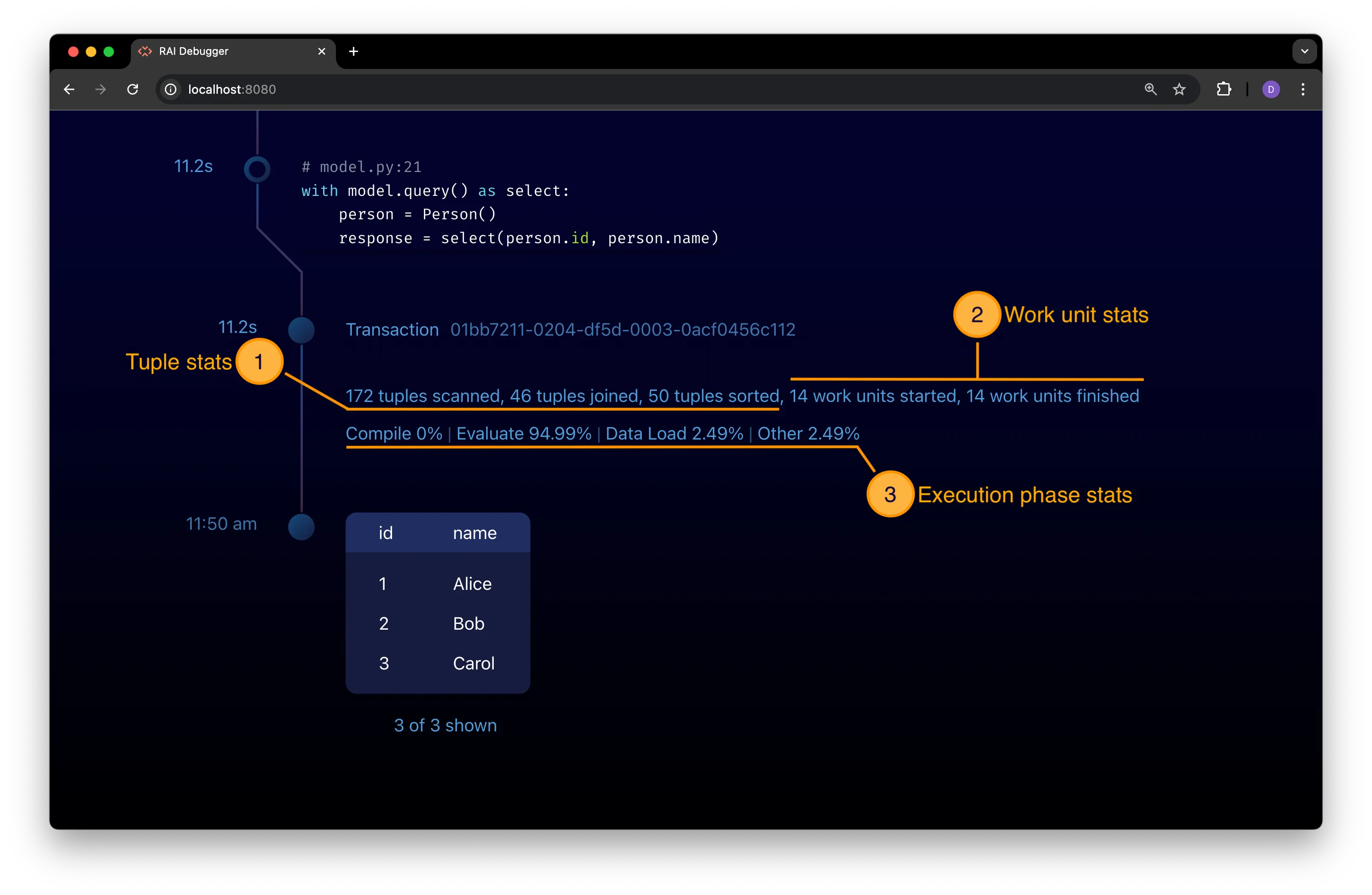
Knowing how to interpret these stats can help you identify potential performance issues in your program.

Use the tabs below to learn more about the different types of stats:

1. Tuples

Interpret Tuple Stats

A tuple is a row of relational data generated by the RAI engine during the execution of a transaction. The compact profile view (see preceding figure) shows you the:

• Total number of tuples scanned—or, generated—during the transaction.
• Number of join operations performed.
• Number of tuples that had to be sorted.

The number of tuples generated by a program is a function of both the number of rows in the source data and the complexity of the rules evaluated by the program. This number can be very large, even if the source data is small.

Look out for transactions with many joins or sorts relative to the total number of tuples. This indicates that the transaction is doing a lot of work and warrants further investigation.

Tip

In a query transaction, you can view tuple stats broken down by rule to understand which rules are generating the most tuples.

2. Work Units

Interpret Work Unit Stats

Work done by the engine to evaluate the transaction is divided into work units that are executed in parallel. Note that work units are not the same as the CPU cores available to the engine.

The compact transaction view (see preceding figure) shows you the:

• Number of work units started by the transaction.
• Number of those work units that have completed their work.

The key thing to look out for here is work units that never terminate. This may indicate that the program’s rules are recursive and stuck in an infinite loop. If necessary, you can cancel a long-running transaction. You’ll need the transaction ID, which is shown next to the transaction node’s timeline icon.

Tip

In a query transaction, you can view work unit stats broken down by rule for insight into which rules unterminated work units are associated with and where unintentional recursion or other performance bottlenecks might be occurring in your program.

3. Execution Phases

Interpret Execution Phase Stats

Statistics about the execution phase of a transaction are shown in the compact profile view as a percentage of the total time spent in each execution phase.

Four phases are shown:

1. Compilation phase: The time spent compiling the transaction.
2. Evaluation phase: The time spent evaluating the transaction.
3. Data load phase: The time spent loading data for the transaction.
4. Other phase: The time spent on other tasks.

Typically, the evaluation phase dominates the total execution time.

Tip

Transactions dominated by the compilation phase may have rules that are too large or complex. You can view individual compilation details to identify rules that may benefit from being split into smaller, less complex rules.

View Rule Compilation Details

To view compilation details for individual rules, expand the installation node that appears after the rules node in the timeline once the transaction is complete:

Each individual rule is shown with its compile size to the left of the rule’s timeline icon, and the rule’s code to the right of the icon.

The rules are sorted by compile size, with the largest compiled rules at the top of the list to help identify rules that may be too large or complex.

Tip

Just because a rule’s compiled size is large does not mean that it is inefficient.

Use the execution phase stats to check what percentage of execution time is spent in the compilation phase. If compilation dominates execution, it may be worth investigating rules with large compile sizes to see if they can be re-written with less complex logic or split into smaller rules.

View Query Execution Details

To view query execution details broken down by individual rule, expand the query’s transaction node in the timeline:

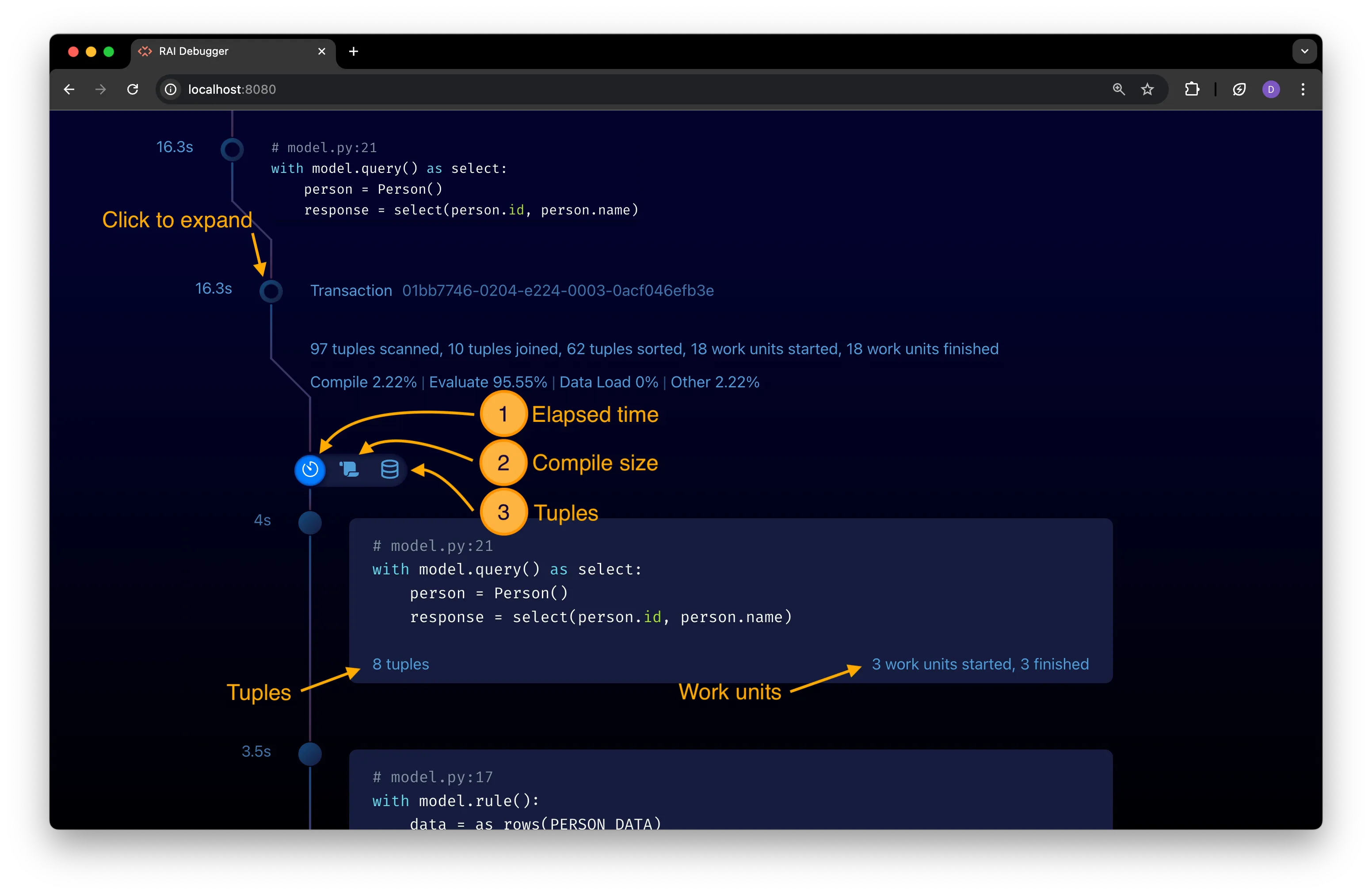
Each individual rule is shown with the:

• Elapsed time to the left of rule’s timeline icon.
• Rule’s code to the right of the icon.
• Tuples processed by the rule during the query’s execution in the bottom left corner.
• Work units started and completed during the rule’s evaluation in the bottom right corner.

By default, rules are sorted by their elapsed execution time, with the longest running rules at the top of the list. Change the sort order by clicking on one of the icons in the menu (see preceding figure) just below the transaction node:

1. Elapsed time: The total elapsed time that the rule took to execute. Sort by this to identify the rules that took the longest to evaluate.

2. Compile size: The size in bytes of the compiled IR for rule. Sort by this to identify the largest compiled rules. See View Rule Compilation Details for more details on interpreting this stat.

3. Tuples: The number of tuples processed by the rule during the query’s execution. Use this view to identify rules that require computing large amounts of data.

Interpret Cross Product Warnings

Cross products are identified by the debugger. Expand a query’s transaction node to view query execution details. Look for a rule with a warning icon in the bottom right corner of the rule’s code block, like in the following figure:

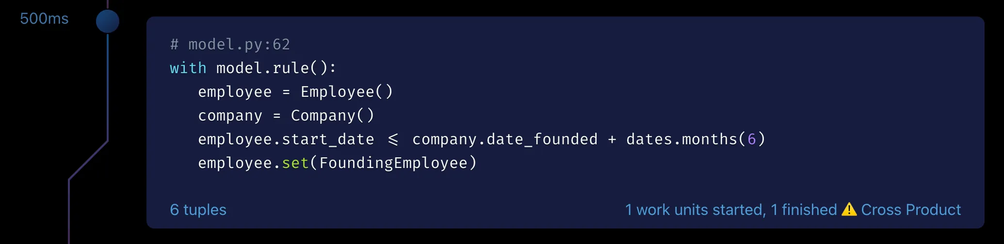
A cross product, also known as a Cartesian product, occurs when two or more variables in a rule or query are not related to each other in any way. This forces the RAI engine to generate all possible combinations of values for the variables. Large cross products can have a significant impact on performance.

Caution

Given the performance implications, cross product warnings should only be ignored if the cross product is intentional.

The rule in the preceding figure has a cross product because every pair of employee and company entities must be generated in order to evaluate the rule. In this case, it’s a logical error, and the rule should be edited to remove the cross product:

# To fix the cross product, add a condition to relate the employee and company:
with model.rule():
   employee = Employee()
   company = Company()
   employee.company_id == company.id  # <-- Add condition to relate employee and company
   employee.start_date <= company.date_founded + dates.months(6)
   employee.set(FoundingEmployee)

# Or, alternatively, reference the employee's company property directly:
with model.rule():
   employee = Employee()
   employee.start_date <= employee.company.date_founded + dates.months(6)
   employee.set(FoundingEmployee)

Sometimes, cross products arise from rules that operate on independent sets of variables. The following rule sets properties for Employee and Company entities, but the employee and company variables are not related to each other way:

from relationalai.std import dates


# BAD:
# An unnecessary cross product.
with model.rule():
   employee = Employee()
   company = Company()  # <-- No condition to relate employee to company
   employee.set(start_year = dates.year(employee.start_date))
   company.set(founded_year = dates.year(company.date_founded))


# GOOD:
# Independent actions are split into separate rules.
with model.rule():
   employee = Employee()
   employee.set(start_year = dates.year(employee.start_date))

with model.rule():
   company = Company()
   company.set(founded_year = dates.year(company.date_founded))

The cross product in the first rule is unnecessary because the actions on the employee and company variables are independent of each other. Logically, the rule is correct, but all possible pairs of employee and company entities must be generated to evaluate the rule. When split into two separate rules, the same effect is achieved without a cross product.

Tip

Cross products in complex rules can have a significant impact on performance. Keep an eye out for the cross product warning in the debugger to help catch these issues early.

Whenever possible, cross products should be removed from rules by:

• Adding conditions to relate the variables to each other, or
• Splitting the rule into multiple, independent rules.