JSON Data With a Data-Defined Schema

This concept guide explains how to work with JSON data that have a data-defined schema, using Rel.

Introduction

This guide describes the data-defined schema representation for JSON data. It also explains how to load data with a data-defined schema, using the built-in Rel relation load_json, and covers running queries, conducting basic exploratory data analysis (EDA), manipulating, and visualizing data.

If you are using a general schema, see the JSON Data With a General Schema guide.

See also the JSON Import and JSON Export guides to learn about importing and exporting JSON data.

Schema Representation

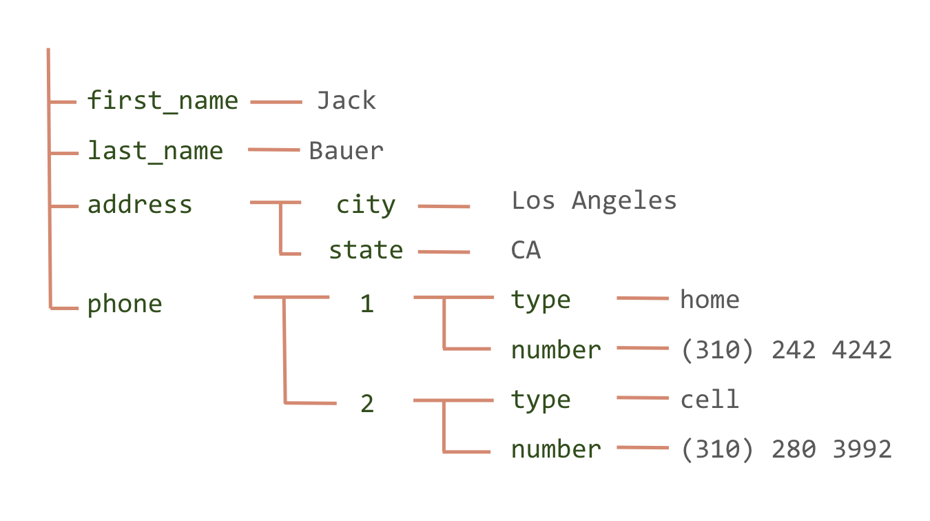
Using the data-defined schema approach, the system extracts the schema from your data and stores each value of the JSON data as a single row in the target relation. For example, consider the following JSON data:

{
    "first_name": "Jack",
    "last_name": "Bauer",
    "address": 
    { 
        "city": "Los Angeles",
        "state": "CA" 
    },
    "phone": 
    [
        { 
            "type": "home",
            "number": "(310) 242 4242" 
        },
        { 
            "type": "cell",
            "number": "(310) 280 3992" 
        }
    ]
}

Here’s their representation using a tree structure:

To load these data using the schema within it, you need to use the built-in Rel relation load_json:

// read query
 
def my_json = load_json["azure://raidocs.blob.core.windows.net/working-with-json/tiny-json.json"]
def output = my_json

Note how the system stores each value of the JSON tree as a single row in the relation my_json.

When there are arrays within your data, the :[] symbol is used as the relation name, immediately followed by an integer. The integer indicates the position of the remaining items within the array. Nested arrays are supported.

💡

When working with a data-defined schema, the RKGS extracts the schema from the data and stores them in a wide format. This means that each key within the JSON data has its respective values and children arranged in a wide relation.

Importing and Exporting JSON Data

Dataset

The remainder of this guide uses the carts.json dataset from DummyJSON (opens in a new tab). This contains information about 20 shopping carts, with each cart containing five products. The dataset also includes information about each product’s name, price, discount, and quantity bought.

Importing Data

💡

To load data using a data-defined schema, use the Rel relation load_json.

You can import and store the example dataset as the base relation my_json as follows:

// write query
 
def insert:my_json = load_json["azure://raidocs.blob.core.windows.net/datasets/carts/carts.json"]
 
def output = my_json

See the JSON Import guide for more details.

Exporting Data

You can export JSON data represented by the data-defined schema using export_json. See the JSON Export guide for more details.

Querying Data

You can use Rel to query data. The following sections contain examples of how to run queries over the example dataset, loaded using a data-defined schema approach.

Filtering Keys

You can select which columns to display. Here’s an example showing only the values of the total and discountedTotal columns from each cart:

// read query
 
module json_data
    def price_discount(cart_id, total, discounted_total) {
        exists(row:
            my_json:carts(:[], row, :id, cart_id) and
            my_json:carts(:[], row, :total, total) and
            my_json:carts(:[], row, :discountedTotal, discounted_total)
        )
    }
end
 
def output = json_data:price_discount

Filtering Values

You can filter values within one key or within multiple keys.

Filtering Within One Key

Say you want to find the carts whose total price is less than 1000:

// read query
 
module json_data
    def less_than_1K(cart_id, total) {
        exists(row:
            my_json:carts(:[], row, :id, cart_id) and
            my_json:carts(:[], row, :total, total) and
            total < 1000
        )
    }
end
 
def output = json_data:less_than_1K

The output of the query has two columns. The first is the ID of the cart and the second is the total price:

Filtering Within Multiple Keys

For this example, say you want to find all the carts that have a total price of less than 1000 but whose discounted price is more than 400:

// read query
 
module json_data
    def pr_lt1K_dp_gt_400(cart_id, total, discounted_total) {
        exists(row:
            my_json:carts(:[], row, :id, cart_id) and
            my_json:carts(:[], row, :total, total) and
            my_json:carts(:[], row, :discountedTotal, discounted_total) and
            total < 1000 and
            discounted_total > 400
        )
    }
end
 
def output = json_data:pr_lt1K_dp_gt_400

The output of the query has three columns. The first is the ID of the cart, the second is total price, and the third is the discounted price:

Using Aggregations and Group-By

Rel also supports aggregate queries over JSON data. Here’s an example that displays the number of purchased items per cart:

// read query
 
module json_data
    def cart_product_quantity(cart_id, product_id, quantity) {
        exists(row1, row2:
            my_json:carts(:[], row1, :id, cart_id) and
            my_json:carts(:[], row1, :products, :[], row2, :id, product_id) and
            my_json:carts(:[], row1, :products, :[], row2, :quantity, quantity)
        )
    }
 
    def quantity_per_cart[cart_id] {
        sum[cart_product_quantity[cart_id, product_id] for product_id]
    }
end
 
def output = json_data:quantity_per_cart

You can also find the product IDs of the least expensive products:

// read query
 
module json_data
    def product_price(product_id, price) {
        exists(row1, row2:
            my_json:carts(:[], row1, :products, :[], row2, :id, product_id) and
            my_json:carts(:[], row1, :products, :[], row2, :price, price)
        )
    }
end
 
def output(p) {
    argmin(json_data:product_price, p)
}

Exploring Data

The imported relation my_json is essentially a Rel module. You can now explore the data using some examples.

Using Tabular Form

One useful way to look at the data is by using the table relation:

// model
 
module table_data
    def totalPrice(cart_id, price) {
        exists(row:
            my_json:carts(:[], row, :id, cart_id) and
            my_json:carts(:[], row, :total, price)
        )
    }
 
    def totalProducts(cart_id, totalProducts) {
        exists(row:
            my_json:carts(:[], row, :id, cart_id) and
            my_json:carts(:[], row, :totalProducts, totalProducts)
        )
    }
 
    def discountedTotal(cart_id, discountedTotal) {
        exists(row:
            my_json:carts(:[], row, :id, cart_id) and
            my_json:carts(:[], row, :discountedTotal, discountedTotal)
        )
    }
 
    def totalQuantity(cart_id, totalQuantity) {
        exists(row:
            my_json:carts(:[], row, :id, cart_id) and
            my_json:carts(:[], row, :totalQuantity, totalQuantity)
        )
    }
end

// read query
 
def output = table[table_data]

You can also select which columns you want to display in a tabular format. Here’s an example showing only the values of the totalProducts and discountedTotal columns:

// read query
 
def output = table[table_data[col] for col in {:totalProducts; :discountedTotal}]

This is the familiar tabular — or unstacked — format of the data. Essentially, table displays the GNF relation table_data as a wide table.

Examining Data

You can now start examining some snippets of the data. The following code displays the user ID of the person who purchased the items in each cart:

// read query
 
module json_data
    def user_id(cart_id, userId) {
        exists(row:
            my_json:carts(:[], row, :id, cart_id) and
            my_json:carts(:[], row, :userId, userId)
        )
    }
end
 
def output = json_data:user_id

Similarly, you can also compute the discount given to each cart:

// read query
 
module json_data
    def discounts(cart_id, discount) {
        exists(row, total_price, discounted_total:
            my_json:carts(:[], row, :id, cart_id) and
            my_json:carts(:[], row, :total, total_price) and
            my_json:carts(:[], row, :discountedTotal, discounted_total) and
            discount = discounted_total / total_price
        )
    }
end
 
def output = json_data:discounts

Finding Outliers

Rel allows you to explore specific columns of the data. For example, sort, and its counterpart reverse_sort, are higher-order relations that sort data. Combining sort with top and bottom allows you to perform a simple data exploration that can help identify outliers.

Here is an example showing the top five most expensive products:

// read query
 
module json_data
    def product_name(cart_id, product_id, title) {
        exists(row1, row2:
            my_json:carts(:[], row1, :id, cart_id) and
            my_json:carts(:[], row1, :products, :[], row2, :id, product_id) and
            my_json:carts(:[], row1, :products, :[], row2, :title, title)
        )
    }
 
    def total_price(cart_id, product_id, total_price) {
        exists(row1, row2:
            my_json:carts(:[], row1, :id, cart_id) and
            my_json:carts(:[], row1, :products, :[], row2, :id, product_id) and
            my_json:carts(:[], row1, :products, :[], row2, :total, total_price)
        )
    }
 
    def key = enumerate[json_data:product_name(cart_id, product_id, _) for cart_id, product_id]
 
    def data_to_show:product_name(key, val) {
        exists(cart_id, product_id:
            json_data:product_name(cart_id, product_id, val) and
            json_data:key(key, cart_id, product_id)
        )
    }
 
    def data_to_show:total_price(key, val) {
        exists(cart_id, product_id:
            json_data:total_price(cart_id, product_id, val) and
            json_data:key(key, cart_id, product_id)
        )
    }
end
 
@ondemand @outline
def top_rows[k, R](col, row, val) {
    exists(order:
        R(col, row, val)
        and sort[second[R]](order, row)
        and order <= k
    )
}
 
def output = table[top_rows[5, json_data:data_to_show]]

Visualizing Data

Rel includes certain built-in functionality to visualize JSON data.

The view_json relation displays a Rel relation as a JSON object represented in the data-defined schema.

For instance, you can visualize the relation person as follows:

// read query
 
def person = load_json["azure://raidocs.blob.core.windows.net/working-with-json/tiny-json.json"]
def output = view_json[person]

For more complex visualizations, Rel provides the Vega-Lite (opens in a new tab) library. For example, you can plot a histogram of the total number of items sold for each product.

The Vega-Lite library requires the data to be in a slightly different form. More specifically, after you set up the necessary data in the relation you want to plot, you need to number the data consecutively. You can do this using the lined_csv functionality. Second, the Vega-Lite library requires that the data be in array format.

In the first example, you will create a horizontal bar chart that shows the total number of times that each product was purchased over the first five carts. Here is the code that creates this plot:

// read query
 
module my_data_bar
    def product_name(cart_id, product_id, title) {
        exists(row1, row2:
            my_json:carts(:[], row1, :id, cart_id) and
            my_json:carts(:[], row1, :products, :[], row2, :id, product_id) and
            my_json:carts(:[], row1, :products, :[], row2, :title, title)
        )
    }
 
    def quantity(cart_id, product_id, quantity) {
        exists(row1, row2:
            my_json:carts(:[], row1, :id, cart_id) and
            my_json:carts(:[], row1, :products, :[], row2, :id, product_id) and
            my_json:carts(:[], row1, :products, :[], row2, :quantity, quantity)
        )
    }
 
    def cp_key = enumerate[product_name(cart_id, product_id, _) for cart_id, product_id]
 
    def data_to_plot:product_name(key, val) {
        exists(cart_id, product_id:
            product_name(cart_id, product_id, val) and
            cp_key(key, cart_id, product_id) and
            cart_id <= 5
        )
    }
 
    def data_to_plot:quantity(key, val) {
        exists(cart_id, product_id:
            quantity(cart_id, product_id, val) and
            cp_key(key, cart_id, product_id) and
            cart_id <= 5
        )
    }
 
    def my_data_graph[:[], i, col] = my_data_bar:data_to_plot[col, i]
end
 
// Assign the data.
def chart:data:values = my_data_bar:my_data_graph
 
// Set up the chart.
def chart:mark:type = "bar"
def chart:mark:tooltip = boolean_true
 
def chart = vegalite_utils:y[{
  (:field, "product_name");
  (:title, "Product Name");
  (:type, "ordinal");
  (:axis, {
    //(:labelAngle, 45);
    (:ticks, boolean_true);
    (:grid, boolean_true);
  })
}]
 
def chart = vegalite_utils:x[{
  (:field, "quantity");
  (:aggregate, "sum");
  (:type, "quantitative");
}]
 
// Display.
def output = vegalite:plot[chart]

The next example creates a scatter plot that shows the total price paid for each product as well as its discounted price. It also computes the discount and considers two groups: one with discounts of more than 10% and one with discounts of 10% or less.

Here is the code that displays this scatter plot:

// read query
 
module my_data_scatter
    def discounted_price(cart_id, product_id, discountedPrice) {
        exists(row1, row2:
            my_json:carts(:[], row1, :id, cart_id) and
            my_json:carts(:[], row1, :products, :[], row2, :id, product_id) and
            my_json:carts(:[], row1, :products, :[], row2, :discountedPrice, discountedPrice)
        )
    }
 
    def total_price(cart_id, product_id, totalPrice) {
        exists(row1, row2:
            my_json:carts(:[], row1, :id, cart_id) and
            my_json:carts(:[], row1, :products, :[], row2, :id, product_id) and
            my_json:carts(:[], row1, :products, :[], row2, :total, totalPrice)
        )
    }
 
    def discount_value(cart_id, product_id, discountPercentage) {
        exists(row1, row2:
            my_json:carts(:[], row1, :id, cart_id) and
            my_json:carts(:[], row1, :products, :[], row2, :id, product_id) and
            my_json:carts(:[], row1, :products, :[], row2, :discountPercentage, discountPercentage)
        )
    }
 
    def cp_key =
        enumerate[discounted_price(cart_id, product_id, _) for cart_id, product_id]
 
    def data_to_plot:discounted_price(key, val) {
        exists(cart_id, product_id:
            discounted_price(cart_id, product_id, val) and
            cp_key(key, cart_id, product_id) and
            val < 200
        )
    }
 
    def data_to_plot:total_price(key, val) {
        exists(cart_id, product_id:
            total_price(cart_id, product_id, val) and
            cp_key(key, cart_id, product_id)
        )
    }
 
    def data_to_plot:discount_value(key, ">10\%") {
        exists(cart_id, product_id, val:
            discount_value(cart_id, product_id, val)  and
            cp_key(key, cart_id, product_id) and
            val > 10
        )
    }
 
    def data_to_plot:discount_value(key, "<=10\%") {
        exists(cart_id, product_id, val:
            discount_value(cart_id, product_id, val) and
            cp_key(key, cart_id, product_id)
            and val <= 10
        )
    }
 
    def my_data_graph[:[], i, col] = data_to_plot[col, i]
end
 
// read query
 
// Assign the data.
def chart:data:values = my_data_scatter:my_data_graph
 
// Set up the chart.
def chart:mark = "point"
 
def chart = vegalite_utils:x[{
  (:field, "discounted_price");
  (:title, "Discounted Price");
  (:type, "quantitative");
  (:scale, :zero, boolean_false);
}]
 
def chart = vegalite_utils:y[{
  (:field, "total_price");
  (:title, "Total Price");
  (:type, "quantitative");
  (:scale, :zero, boolean_false);
}]
 
def chart = vegalite_utils:color[{
  (:field, "discount_value");
  (:type, "nominal");
  (:scale, :domain, :[], {(1, ">10\%"); (2, "<=10\%")});
  (:title, "Discount");
 
}]
 
// Display.
def output = vegalite:plot[chart]

Summary

You have learned how to work with JSON data represented by a data-defined schema using Rel, including loading, exploring, manipulating and visualizing them.

See the JSON Import and JSON Export guides to learn about importing and exporting JSON data.

Was this doc helpful?