JSON Data With a General Schema

This concept guide explains how to work with JSON data that have a general schema, using Rel.

Introduction

This guide describes the general schema representation for JSON data. It also explains how to load data with a general schema, using the built-in Rel relation load_json_general, and covers running queries, conducting basic exploratory data analysis (EDA), manipulating, and visualizing data.

If you are working with a data-defined schema, see the JSON Data With a Data-Defined Schema guide.

See also the JSON Import and JSON Export guides to learn about importing and exporting JSON data.

Schema Representation

Using the general schema approach, the system stores the JSON data as a tree, the nodes of which are treated as entities. Each entity is represented by a unique ID (a Hash).

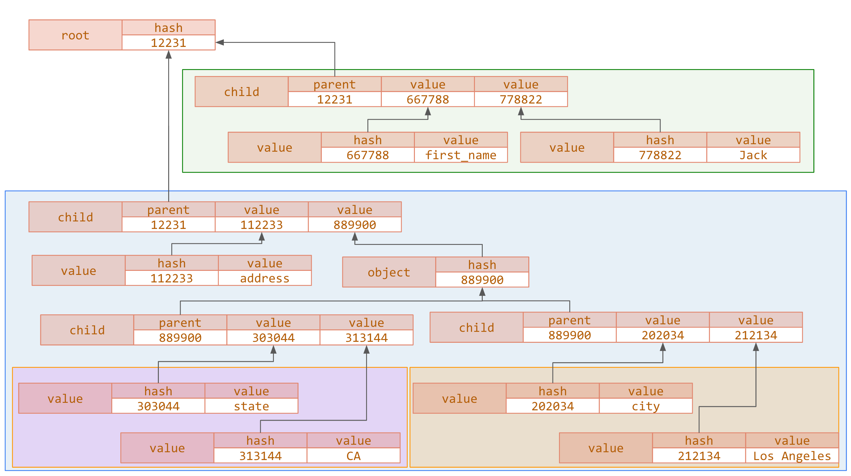
For example, consider the following data:

{
  "first_name": "Jack",
  "address": { "city": "Los Angeles",
               "state": "CA" }
}

Here’s their representation using a tree with different levels — the name (green portion), the address (blue portion), the city (orange portion), and the state (purple portion):

This representation creates relations with more rows than the data-defined approach. These are the relations used in this representation:

Relation	Schema	Description
`root`	`Hash`	This relation is the outermost level of a JSON file. It is usually a JSON object.
`value`	`(Hash, <value>)`	This relation captures actual stored data. The field `<value>` represents one of the supported JSON data types. For instance, `String` or `Int64`.
`array`	`Hash`	This relation captures JSON arrays and can be used to distinguish an empty array from an empty object.
`object`	`Hash`	This relation captures JSON objects. In a given JSON file, identical subtrees use the same entity.
`child`	`(Hash, Hash, Hash)`	This relation `(node1, node2, node3)` captures node relationships. The node `node 1` is the parent node, `node2` serves as the name for objects or the index for arrays, and `node3` is the child node.
`index`	`(Hash, Hash, Hash)`	This relation `(conn, node, root)` establishes a connection from each node (value, object, or array) with the `root` node. The field `conn` is the connection ID, `node` is any node in the JSON tree, and the third field is always the `root` node.

See the example below to better understand each relation.

Although this approach may seem elaborate, it is generic and allows for better scaling. Essentially, each relation has a “pointer” — in terms of an entity ID — that points to the parent nodes in the JSON tree.

💡

When working with a general schema, the RKGS stores the JSON data as a tree, the nodes of which are treated as entities.

To load JSON data with a general schema, you have to use the Rel relation load_json_general. This is useful for cases that require JSON data of arbitrary depth. In this case, load_json_general allows you to load such data without any scaling issues, even when there are several distinct property names in the data.

Example

Consider the following JSON data:

{
    "first_name": "Jack",
    "last_name": "Bauer",
    "address":
    {
        "city": "Los Angeles",
        "state": "CA"
    },
    "phone":
    [
        {
            "type": "home",
            "number": "(310) 242 4242"
        },
        {
            "type": "cell",
            "number": "(310) 280 3992"
        }
    ]
}

Here’s an example that loads them using a general schema:

// write query
 
def insert:my_json_general_schema = load_json_general["azure://raidocs.blob.core.windows.net/working-with-json/tiny-json.json"]
 
def output = my_json_general_schema

Each individual node in the JSON tree is represented in a separate row.

The relation root looks like this:

// read query
 
with my_json_general_schema use root
 
def output = root

You can get the rest of the relations in a similar way:

// read query
 
with my_json_general_schema use value, child, root, array, object, index
 
def output:child = child
def output:value = value
def output:array = array
def output:object = object
def output:index = index

To work with the general schema you can use Rel joins.

Here’s an example that queries the two phone numbers in the data:

// read query
 
with my_json_general_schema use value, child, root
 
def array_indexes[v, x] = value(x, v) and Int(v)
def name[s, x] = value(x, s) and String(s)
 
def phones[id] = root.child[name["phone"]].child[array_indexes[id]].child[name["number"]].value
 
def output = phones

Importing and Exporting JSON Data

Dataset

This guide uses the carts.json dataset from DummyJSON (opens in a new tab). This contains information about 20 shopping carts, with each cart containing five products. The dataset also includes information about each product’s name, price, discount, and quantity bought.

Importing Data

💡

To load data using a general schema, use the Rel relation load_json_general.

You can import and store the example dataset as the base relation my_json_general as follows:

// write query
 
def insert:my_json_general = load_json_general["azure://raidocs.blob.core.windows.net/datasets/carts/carts.json"]
 
def output = my_json_general

This guide uses the installed model below. The relation array_indexes defines the arrays contained within the JSON data, while the relation name defines the key names:

// model
 
with my_json_general use value, child, root
 
def array_indexes[v, x] = value(x, v) and Int(v)
def name[s, x] = value(x, s) and String(s)

See the JSON Import guide for more details.

Exporting Data

Exporting data using the general schema is not currently supported. You can only export using the data-defined schema.

See the JSON Export guide for more details.

Querying Data

You can use Rel to query data. The following sections contain examples of how to run queries over the sample dataset, loaded using a general schema approach.

Filtering Keys

You can select which columns to display. Here’s an example showing only the values of the total and discountedTotal columns from each cart:

// read query
 
with my_json_general use value, child, root
 
module json_data
    def total_price[cart_id] {
        root.child[name["carts"]].child[array_indexes[cart_id]].child[name["total"]].value
    }
 
    def discounted_total[cart_id] {
        root.child[name["carts"]].child[array_indexes[cart_id]].child[name["discountedTotal"]].value
    }
 
    def price_discount(cart_id, tp, dt) {
        total_price(cart_id, tp) and
        discounted_total(cart_id, dt)
    }
end
 
def output = json_data:price_discount

Filtering Values

You can filter values within one key or within multiple keys.

Filtering Within One Key

As a first example, say you want to find the carts whose total price is less than 1000:

// read query
 
with my_json_general use value, child, root
 
module json_data
    def total_price[cart_id] {
        root.child[name["carts"]].child[array_indexes[cart_id]].child[name["total"]].value
    }
 
    def less_than_1K(cart_id, tp) {
        total_price(cart_id, tp) and
        tp < 1000
    }
end
 
def output = json_data:less_than_1K

The output of the query has two columns. The first is the ID of the cart and the second is the total price:

Filtering Within Multiple Keys

For this example, say you want to find all the carts that have a total price of less than 1000 but whose discounted price is more than 400:

// read query
 
with my_json_general use value, child, root
 
module json_data
    def total_price[cart_id] {
        root.child[name["carts"]].child[array_indexes[cart_id]].child[name["total"]].value
    }
 
    def discounted_total[cart_id] {
        root.child[name["carts"]].child[array_indexes[cart_id]].child[name["discountedTotal"]].value
    }
 
    def pr_lt1K_dp_gt_400(cart_id, tp, dt) {
        total_price(cart_id, tp) and
        discounted_total(cart_id, dt) and
        tp < 1000 and
        dt > 400
    }
end
 
def output = json_data:pr_lt1K_dp_gt_400

The output of the query has three columns. The first is the ID of the cart, the second is the total price, and the third is the discounted price:

Essentially, each query that involves multiple keys is effectively a join between the separate relations that contain the respective data.

Using Aggregations and Group-By

Rel also supports aggregate queries over JSON data. Here’s an example that displays the number of purchased items per cart:

// read query
 
with my_json_general use value, child, root
 
module json_data
    def cart_product_quantity[cart_id, product_id] {
        root.child[name["carts"]].child[array_indexes[cart_id]].child[name["products"]].child[array_indexes[product_id]].child[name["quantity"]].value
    }
 
    def quantity_per_cart[cart_id] {
        sum[cart_product_quantity[cart_id, product_id] for product_id]
    }
end
 
def output = json_data:quantity_per_cart

You can also find the product IDs of the least expensive products:

// read query
 
with my_json_general use value, child, root
 
module json_data
    def id[cart_id, id] {
        root.child[name["carts"]].child[array_indexes[cart_id]].child[name["products"]].child[array_indexes[id]].child[name["id"]].value
    }
 
    def price[cart_id, id] {
        root.child[name["carts"]].child[array_indexes[cart_id]].child[name["products"]].child[array_indexes[id]].child[name["price"]].value
    }
 
    def product_price(product_id, price) {
        exists(cart_id, id:
            json_data:id(cart_id, id, product_id) and
            json_data:price(cart_id, id, price)
        )
    }
end
 
def output(p) {
    argmin(json_data:product_price, p)
}

Exploring Data

The imported relation my_json_general is essentially a Rel module. You can now explore the data using some examples.

Using Tabular Form

One useful way to look at the data is by using the table relation:

// model
 
with my_json_general use value, child, root
 
module table_data
    def totalPrice[cart_id] {
        root.child[name["carts"]].child[array_indexes[cart_id]].child[name["total"]].value
    }
 
    def totalProducts[cart_id] {
        root.child[name["carts"]].child[array_indexes[cart_id]].child[name["totalProducts"]].value
    }
 
    def discountedTotal[cart_id] {
        root.child[name["carts"]].child[array_indexes[cart_id]].child[name["discountedTotal"]].value
    }
 
    def totalQuantity[cart_id] {
        root.child[name["carts"]].child[array_indexes[cart_id]].child[name["totalQuantity"]].value
    }
end

// read query
 
def output = table[table_data]

You can also select which columns you want to display in a tabular format. Here’s an example showing only the values of the totalProducts and discountedTotal columns:

// read query
 
def output = table[table_data[col] for col in {:totalProducts; :discountedTotal}]

This is the familiar tabular — or unstacked — format of the data. Essentially, table displays the GNF relation table_data as a wide table.

Examining Data

You can now start examining some snippets of the data. The following code displays the user ID of the person who purchased the items in each cart:

// read query
 
with my_json_general use value, child, root
 
module json_data
    def user_id[cart_id] {
        root.child[name["carts"]].child[array_indexes[cart_id]].child[name["userId"]].value
    }
end
 
def output = json_data:user_id

Similarly, you can also compute the discount given to each cart:

// read query
 
with my_json_general use value, child, root
 
module json_data
    def discounts(cart_id, discount) {
        exists(total_price, discounted_total:
            root.child[name["carts"]].child[array_indexes[cart_id]].child[name["total"]].value(total_price) and
            root.child[name["carts"]].child[array_indexes[cart_id]].child[name["discountedTotal"]].value(discounted_total) and
            discount = discounted_total / total_price
        )
    }
end
 
def output = json_data:discounts

Finding Outliers

Rel allows you to explore specific columns of the data. For example, sort, and its counterpart reverse_sort, are higher-order relations that sort data. Combining sort with top and bottom allows you to perform a simple data exploration that can help identify outliers.

Here is an example showing the top five most expensive products:

// read query
 
with my_json_general use value, child, root
 
module json_data
    def product_name[cart_id, product_id] {
        root.child[name["carts"]].child[array_indexes[cart_id]].child[name["products"]].child[array_indexes[product_id]].child[name["title"]].value
    }
 
    def total_price[cart_id, product_id] {
        root.child[name["carts"]].child[array_indexes[cart_id]].child[name["products"]].child[array_indexes[product_id]].child[name["total"]].value
    }
 
    def key = enumerate[json_data:product_name(cart_id, product_id, _) for cart_id, product_id]
 
    def data_to_show:product_name(key, val) {
        exists(cart_id, product_id:
            json_data:product_name(cart_id, product_id, val) and
            json_data:key(key, cart_id, product_id)
        )
    }
 
    def data_to_show:total_price(key, val) {
        exists(cart_id, product_id:
            json_data:total_price(cart_id, product_id, val) and
            json_data:key(key, cart_id, product_id)
        )
    }
end
 
@ondemand @outline
def top_rows[k, R](col, row, val) {
    exists(order:
        R(col, row, val)
        and sort[second[R]](order, row)
        and order <= k
    )
}
 
def output = table[top_rows[5, json_data:data_to_show]]

Visualizing Data

Rel allows you to visualize data using the Vega-Lite (opens in a new tab) library. You can plot different views of data using the various visualization capabilities.

For example, you can plot a histogram of the total number of items sold for each product.

The Vega-Lite library requires the data to be in a slightly different form. More specifically, after you set up the necessary data in the relation you want to plot, you need to number the data consecutively. You can do this using the lined_csv functionality. Second, the Vega-Lite library requires that the data be in array format.

In the first example, you will create a horizontal bar chart that shows the total number of times that each product was purchased over the first five carts. Here is the code that creates this plot:

// read query
 
with my_json_general use value, child, root
 
module my_data_bar
    def product_name[cart_id, product_id] {
        root.child[name["carts"]].child[array_indexes[cart_id]].child[name["products"]].child[array_indexes[product_id]].child[name["title"]].value
    }
 
    def quantity[cart_id, product_id] {
        root.child[name["carts"]].child[array_indexes[cart_id]].child[name["products"]].child[array_indexes[product_id]].child[name["quantity"]].value
    }
 
    def cp_key = enumerate[product_name(cart_id, product_id, _) for cart_id, product_id]
 
    def data_to_plot:product_name(key, val) {
        exists(cart_id, product_id:
            product_name(cart_id, product_id, val) and
            cp_key(key, cart_id, product_id) and
            cart_id <= 5
        )
    }
 
    def data_to_plot:quantity(key, val) {
        exists(cart_id, product_id:
            quantity(cart_id, product_id, val) and
            cp_key(key, cart_id, product_id) and
            cart_id <= 5
        )
    }
 
    def my_data_graph[:[], i, col] = my_data_bar:data_to_plot[col, i]
end
 
// Assign the data.
def chart:data:values = my_data_bar:my_data_graph
 
// Set up the chart.
def chart:mark:type = "bar"
def chart:mark:tooltip = boolean_true
 
def chart = vegalite_utils:y[{
  (:field, "product_name");
  (:title, "Product Name");
  (:type, "ordinal");
  (:axis, {
    //(:labelAngle, 45);
    (:ticks, boolean_true);
    (:grid, boolean_true);
  })
}]
 
def chart = vegalite_utils:x[{
  (:field, "quantity");
  (:aggregate, "sum");
  (:type, "quantitative");
}]
 
// Display.
def output = vegalite:plot[chart]

The next example creates a scatter plot that shows the total price paid for each product as well as its discounted price. It also computes the discount and considers two groups: one with discounts of more than 10% and one with discounts of 10% or less.

Here is the code that displays this scatter plot:

// read query
 
with my_json_general use value, child, root
 
module my_data_scatter
    def discounted_price[cart_id, product_id] {
        root.child[name["carts"]].child[array_indexes[cart_id]].child[name["products"]].child[array_indexes[product_id]].child[name["discountedPrice"]].value
    }
 
    def total_price[cart_id, product_id] {
        root.child[name["carts"]].child[array_indexes[cart_id]].child[name["products"]].child[array_indexes[product_id]].child[name["total"]].value
    }
 
    def discount_value[cart_id, product_id] {
        root.child[name["carts"]].child[array_indexes[cart_id]].child[name["products"]].child[array_indexes[product_id]].child[name["discountPercentage"]].value
    }
 
    def cp_key =
        enumerate[discounted_price(cart_id, product_id, _) for cart_id, product_id]
 
    def data_to_plot:discounted_price(key, val) {
        exists(cart_id, product_id:
            discounted_price(cart_id, product_id, val) and
            cp_key(key, cart_id, product_id) and
            val < 200
        )
    }
 
    def data_to_plot:total_price(key, val) {
        exists(cart_id, product_id:
            total_price(cart_id, product_id, val) and
            cp_key(key, cart_id, product_id)
        )
    }
 
    def data_to_plot:discount_value(key, ">10\%") {
        exists(cart_id, product_id, val:
            discount_value(cart_id, product_id, val)  and
            cp_key(key, cart_id, product_id) and
            val > 10
        )
    }
 
    def data_to_plot:discount_value(key, "<=10\%") {
        exists(cart_id, product_id, val:
            discount_value(cart_id, product_id, val) and
            cp_key(key, cart_id, product_id)
            and val <= 10
        )
    }
 
    def my_data_graph[:[], i, col] = data_to_plot[col, i]
end
 
// read query
 
// Assign the data.
def chart:data:values = my_data_scatter:my_data_graph
 
// Set up the chart.
def chart:mark = "point"
 
def chart = vegalite_utils:x[{
  (:field, "discounted_price");
  (:title, "Discounted Price");
  (:type, "quantitative");
  (:scale, :zero, boolean_false);
}]
 
def chart = vegalite_utils:y[{
  (:field, "total_price");
  (:title, "Total Price");
  (:type, "quantitative");
  (:scale, :zero, boolean_false);
}]
 
def chart = vegalite_utils:color[{
  (:field, "discount_value");
  (:type, "nominal");
  (:scale, :domain, :[], {(1, ">10\%"); (2, "<=10\%")});
  (:title, "Discount");
 
}]
 
// Display.
def output = vegalite:plot[chart]

Summary

You have learned how to work with JSON data represented by a general schema using Rel, including loading, exploring, manipulating, and visualizing them.

See the JSON Import and JSON Export guides to learn about importing and exporting JSON data.

Was this doc helpful?